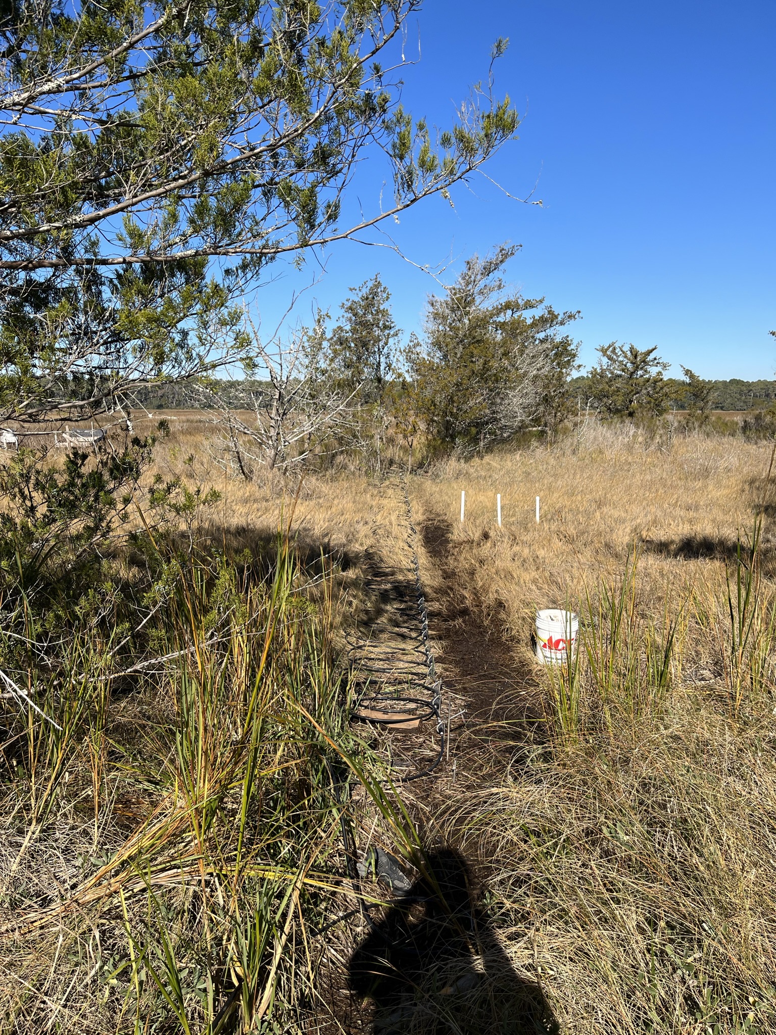
Transect Y, December 2021.
A Master of Science Thesis Project completed in progress towards a degree in Coastal Marine and Wetland Science
The intention of this site is to provide a plain language summary of the project and to share some of the pictures and data gathered along the way. This is a living site with updates as new data emerges, if a section is blank, check back soon!
This site is a non-technical document aiming for greater dissemination of the project's findings, for a concise technical manuscript follow the link above.
Scenery of Waties Island, SC and sights of project data acquisition. Hover over images to see the description.
Transect Y, December 2021.
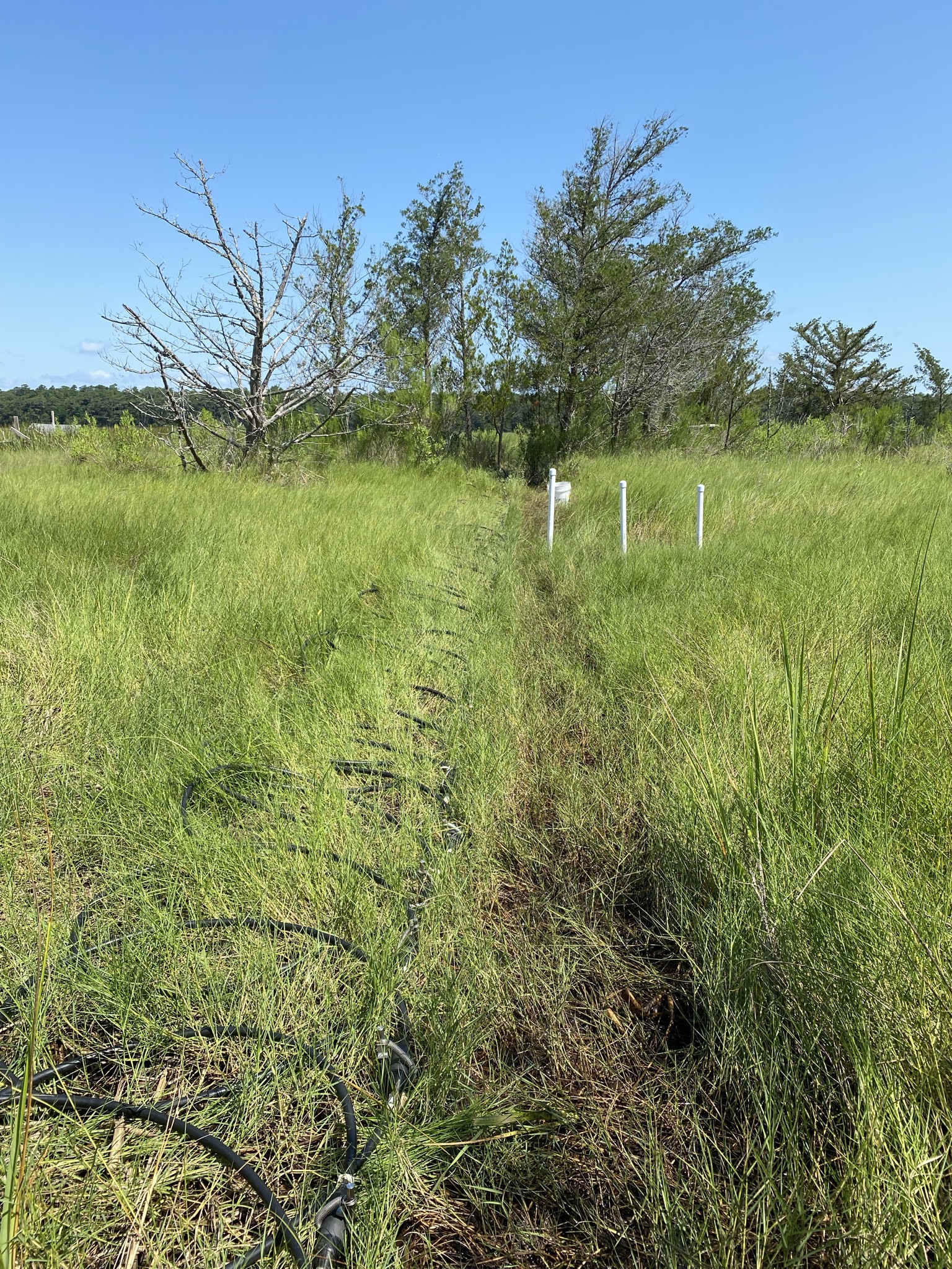
Transect Y, June 2021.

The sun sets over the low marsh well after installation/p>

High tide meets the ER survey

Sea Fog on Transect Y, January 2022.

Vibracore tripod ready to pull Core 5.

Reading ER tomograms in the field.

Wildflowers of Salt Marsh Aster.

Waties Island hammocks as seen from Cherry Grove Beach during a full moon.

An example of sediments excavated using a hand auger during installation of nested wells on Trnasect Y.

ER survey of Transect Y during November 2021

Vibrant stems of Salicornia aka. "Salt Sea Beans" in high marsh salt pans

A twisted loblolly pine

Some exploratory ER work

Iron rich groundwaters flowing out of the barrier island at a steep transition between maritime forest and low marsh

Biofilm near the mixing zone of estuarine and barrier island waters

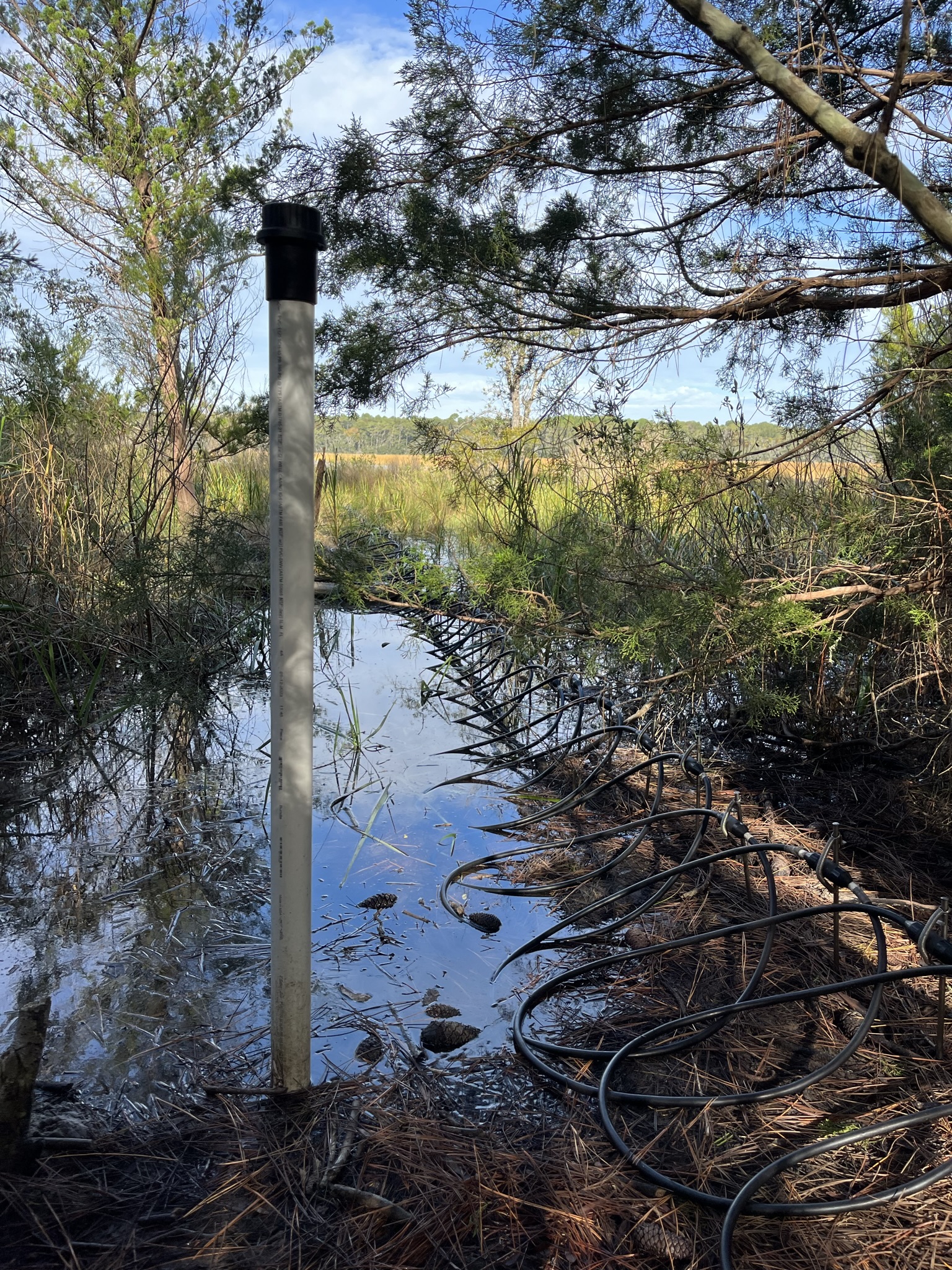
The low marsh well post-installation

Clearing the well of water at high tide

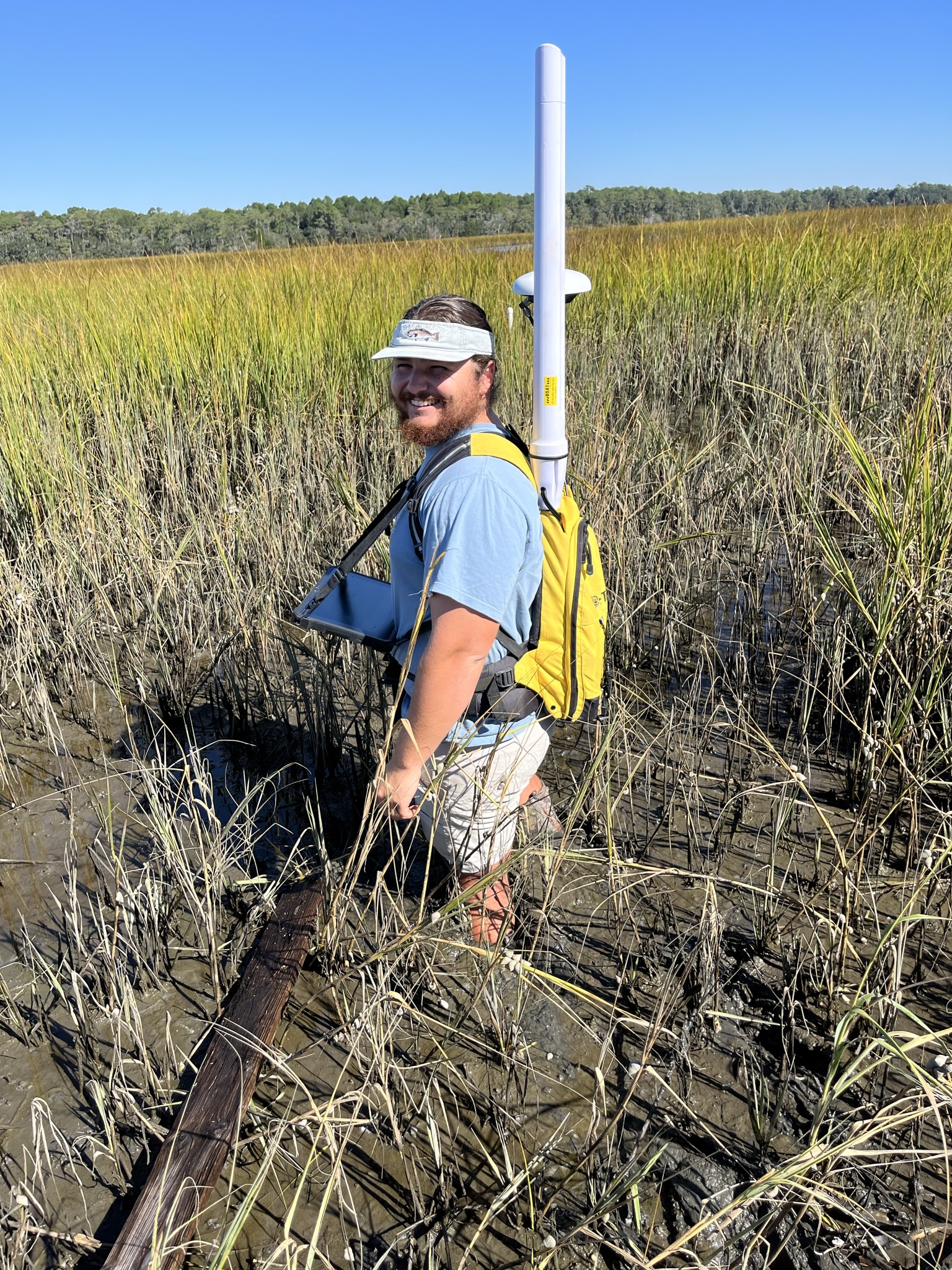
Stuck in the mud while getting elevation data during an RTK survey.

A view of Transect Z

You never know what will wash up on the beach...

Equipment related to crab fishing is some of the most common marine debris at Waties Island

Wind blown sands on the beach face

Rocky outcrops just off the beach frequently foul shrimp trawls along Long Bay

An outrigger from a small shrimp trawler

Knobbed whelks are a common sight on the beach

A Dunn Sound oyster reef

Eden Saltworks Creek with Cherry Grove Beach in the background

Subsampling Core 1

Installation of the nested groundwater wells along Transect Y
South Carolina’s “Grand Strand” is an uninterrupted 60-mile stretch of white sandy beaches, seaside resorts, and golf courses along the state’s northeastern coast. At the northern terminus of this vacation paradise lies Waties Island, an undeveloped barrier island that exists as part of a broader conservation and research easement along the Little River neck.
Waties Island is bound by two inlets, Hog Inlet, which separates the island from Cherry Grove Beach to the south, and Little River Inlet to the north, which serves as the SC-NC state boundary and separates the island from Sunset Beach. The island’s central axis is oriented approximately 72 degrees east of north and is the first in a chain of barrier islands that begin in the northeastern half of Long Bay.
As with most barrier islands in the southeast, the sediments that comprise the island began accumulating 6,000 – 10,000 years ago during the Holocene epoch. This period in geologic time is characterized by rapidly rising sea levels as ice from the last glacial maximum began to melt. While rising seas began to inundate the continental shelf on the east coast around 16,000 years ago, global climate began to stabilize during the Holocene and thus a gentler rise in sea level facilitated the accumulation of coastal sediments into the barrier islands present today.
Small variations in sea level can shift barrier island complexes landward and seaward, known as regressive (island moving offshore) and transgressive (island moving inland) cycles. Evidence of these shifts can be seen in LiDAR imagery of the island where paleo beach ridges and dune fields are observed parallel to the island’s modern coast.
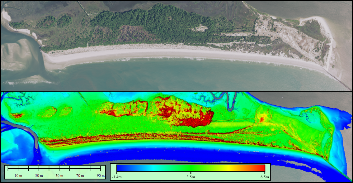
The result of the island’s foundational geology is a mosaic of unique habitats and landscapes including interdunal swale, maritime forest, salt marsh, brackish swamps, and a significant estuarine environment known as Dunn Sound. These environments are created by a combination of geological, hydrological, and ecological factors that allow plant and animal species to become exceptionally adapted to their surroundings. For example, Spartina alterniflora, the species which dominates the lower reaches of saltmarshes tolerates highly saline waters, while woody species which inhabit uplands such as Live oak (Quercus virginiana) and Eastern Red Cedar (Juniperus virginiana) require fresher waters and may experience stress or death when exposed to saltier waters.
If we shift our view of barrier islands away from an ecological perspective and more towards a hydrogeological perspective, the species which inhabit each region of the island can provide clues and insight into the physical characteristics of the geology and groundwater under the surface.
Hydrogeology is a field which deals with the interactions of water and sediment. Often it investigates how inputs and outputs of water interact with the sediment and material in the environment. Examples of hydrogeologic studies could include evaluating how fast stormwater will percolate into a retention pond or monitoring the extraction of groundwater from large aquifers for human use. Most hydrogeologic studies focus on interactions between humans and the environment such as the previously mentioned examples, however there is a growing body of literature investigating how groundwaters interact with the natural environment. The motivation for such studies is to better understand processes that involve groundwaters, such as nutrient exchange, the dissolution of some bedrocks that create sinkholes, or to understand how changes in the hydrologic cycle will affect ecosystems. On barrier islands, hydrogeologic studies often focus on understanding what creates freshwater on the island, and how those fresh waters move and interact with the subterranean environment until they end up in the coastal ocean.
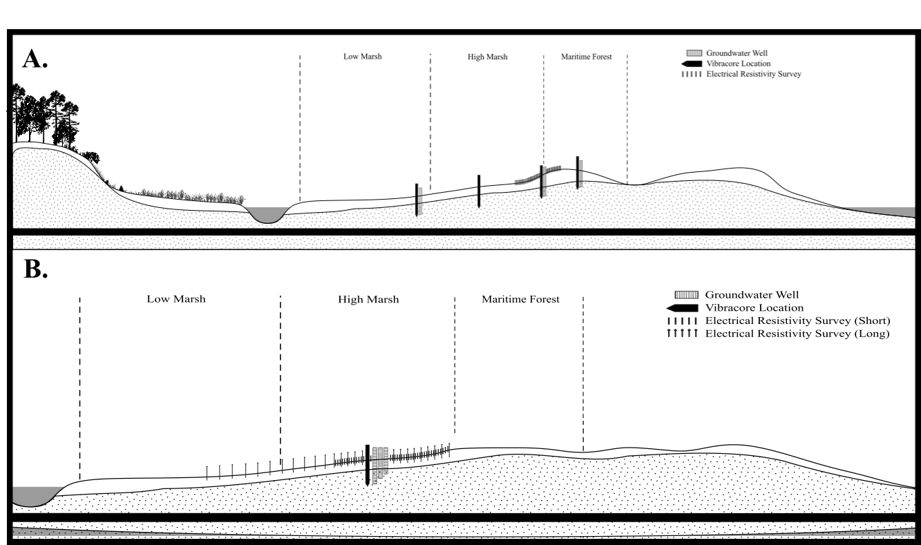
A simplified hydrogeologic model of southeastern barrier islands is pictured below.
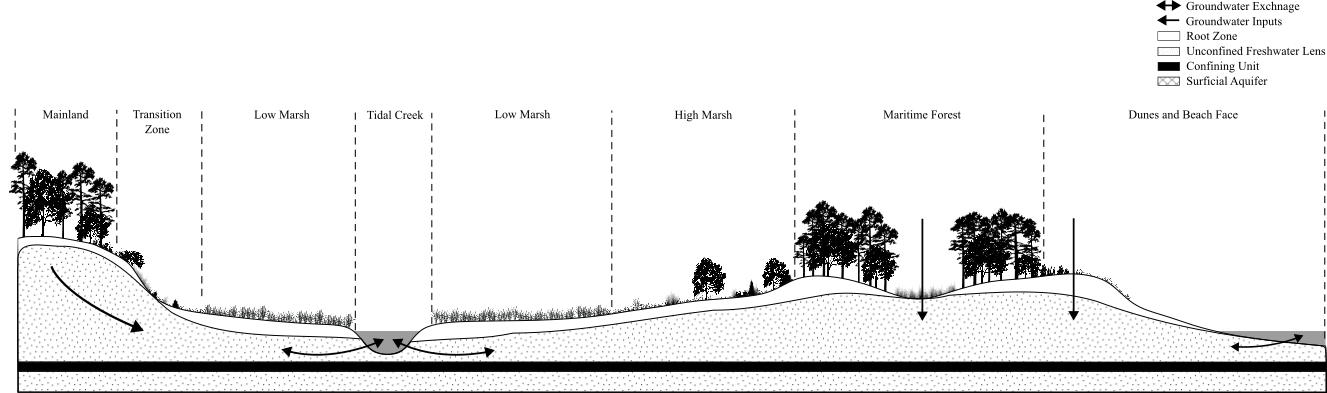
In these environments groundwaters can exist in two basic forms, a traditional aquifer, which is confined between impermeable layers in the earth, known as aquitards, or as a freshwater lens which is a “bubble” of fresh water that may rest atop saltier water or an aquitard. The most common origin of freshwater on barrier islands is from rain or “meteoric waters”. It’s been suggested that sand dunes are the area where this rainwater infiltrates the ground the easiest due to the high permeability of sand. Additionally, this region is typically the highest elevation of a barrier island, resulting in the areas where the water table will be at its highest elevation. This point is often referred to as the top hydraulic head on the island or the point at which groundwaters will flow away due to gravity. From the dunes, groundwater may move towards the ocean through the beach or towards the marsh through the island. The beach face is a known area of groundwater exchange, where freshwaters mix with seawater within the sandy sediments. The alternate path of groundwater is more complex. In the case of Waties Island, fresh water at the dune may drain to the brackish swamp in the core of the island, where the island’s water table is exposed due to low elevation. However, the water table extends into the maritime forest on the landward side of the island where it is used by woody plants and trees. As the elevation of the maritime forest gives way to the salt marsh, groundwater flow becomes increasingly complex. Highly permeable sands in the maritime forest transition into much finer silt and mud typical of the salt marsh. These marsh sediments are notably low permeability soils, blocking the lateral and vertical movement of groundwater. Yet groundwaters are able to continue their flow path towards the marsh. How is this possible? Fine scall geologic differences created by a process known as overwash provide highly permeable “plumbing” for groundwaters to infiltrate the marsh. What is overwash? Overwash occurs when coastal storms or hurricanes create waves significant enough to overtop or erode sand dunes and push those sandy sediments back into the island.
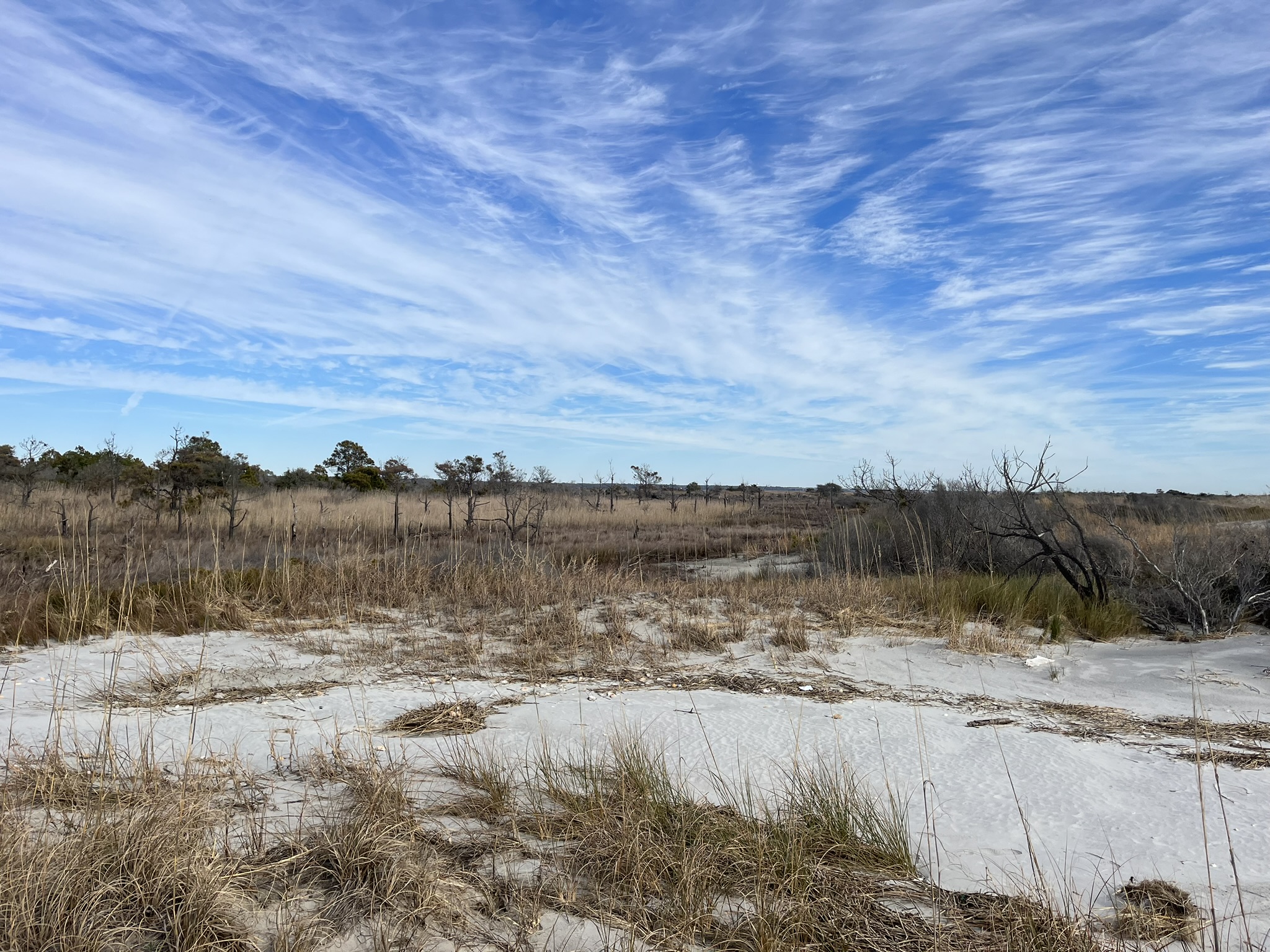
These relic overwash fans exist within the geology of the marsh and result in nonhomogeneous transport and mixing between estuarine and fresh groundwaters in the saltmarsh. We can further complicate this transport by adding factors such as tidal forcing, which can reverse the flow of groundwater at higher tides or accelerate the flow during low tides. Other factors that can affect groundwater flow through the marsh include evapotranspiration, seasonal demands by plants, and of course human modification such as constructing sea walls, roads, or ponds.
The hydrogeologic scene on barrier islands is complex and nuanced, requiring expertise in a variety of fields, so why are studies here important? Understanding the “plumbing” of barrier islands is essential to painting a complete picture of the ecosystem services these environments provide. For example, it may be apparent that a barrier island serves as just that, a barrier to protect coastal communities from the brunt of storm damage and coastal hazards. However, if climactic changes such as sea level rise threaten to increase the amount of salty groundwater in the island, keystone flora such as oak and pine trees may die-off, threatening to destabilize the island and reduce its protective services to coastal communities. Additionally, characterizing and quantifying the groundwaters flowing through the island allows researchers to better understand the importance of groundwater for transporting nutrients from the wetlands of the island into the estuary and coastal ocean, providing foundational nutrition for the food chain in these environments. Barrier island hydrogeological studies can also serve as small-scale experiments and studies for much larger coastal aquifer systems. Saltwater intrusion is one of the foremost threats to the coastal aquifers that supply municipalities and cities with freshwater resources. Increasing sea level increases the force that salty groundwater pushes into freshwater regions on the coastal plain. Coupling this with increasing urbanization and demand for freshwater from these systems creates the potential for widespread salinization of aquifers, diminishing their value as a utility.
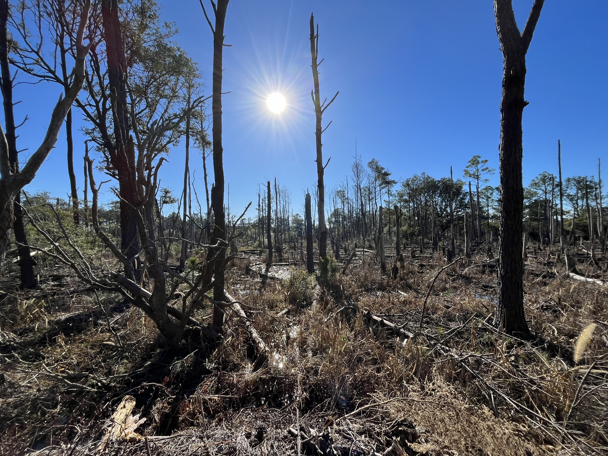
While several studies have focused on studying the interactions of fresh, island groundwater and salty, ocean waters on the beach face or creek bank, few have attempted to characterize the mixing occurring within the transition from maritime forest to salt marsh. Here, the underground mixing of waters should be apparent, as salty water is forced through the marsh sediments by the tide until it reaches the freshwater flowing off the island due to gravity. To characterize the geology and attempt to capture the properties of groundwater as it traverses this boundary, we have to bring the study to a two-dimensional level. To do this we have established three transects or lines where we will study the subsurface of the island.
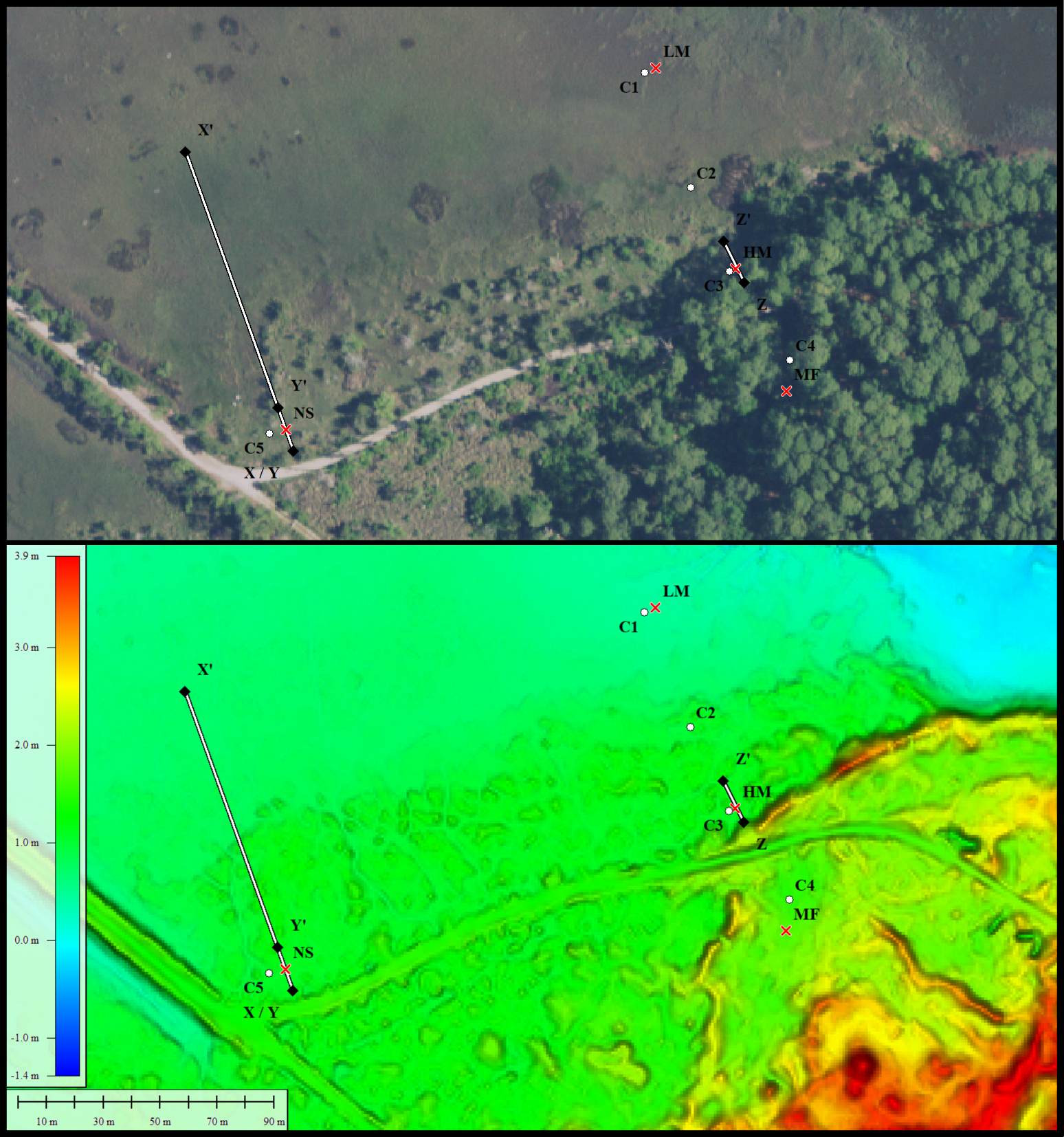
Transect X covers to transition from high elevation to low elevation saltmarsh, transect Y provides high-resolution insight into the high marsh and transect Z spans the transition from maritime forest to high elevation saltmarsh.
Knowing the elevation of the water table through time at different points along the transects not only allows for the characterization of the shape of the water table but also reveals environmental signals, such as tidal forcing or the impact of storms. To get these water table measurements, three groundwater wells were installed along transect Z with one well in each ecological zone, maritime forest, high marsh, and low marsh. The wells are made of 3/4'” PVC pipe with a 2 1/2” interval of slotted screen at the end to allow for groundwater to enter the pipe. At each site, a hole was dug with post-hole diggers until the water table was hit and the hole would begin to collapse. At that point, a larger PVC pipe was inserted to keep the excavation open, and further depth was achieved with a hand auger. Due to the marsh sites containing fine-grained muds and silts that could clog the well screen, the well point was placed in the excavation and backfilled with beach sand to act as a buffer. Each wellpoint was installed into the freshwater lens, aka. water table, so that water table elevations could be recorded. In the center of transect Y a set of smaller wells were installed. Unlike the wells on transect Z these wells were installed in the same location, the center of the transect, but at different depths to evaluate how groundwater characteristics might change within different layers of sediment.
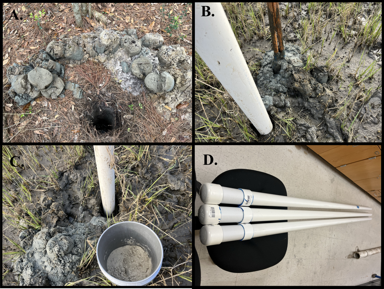
Recognizing the influence that small-scale geologic features such as overwash fans may impose on the flow of groundwater, a robust description of the sediments contained in the study site is needed. To accomplish this, a vibracore is taken. Vibracoring is a method of extracting sediment from the subsurface by attaching a weighted vibrating head to the top of an aluminum core barrel. The vibrating head is powered by a gas engine typically used for finishing concrete. These concrete engines have a fitting that spins a flexible shaft that when used for concrete work, vibrates a screed and provides a fine smooth finish. In a geotechnical setting, rather than a screed, the shaft spins a counterweight that creates intense vibrations along the length of the core barrel. When these vibrations reach the ground, liquefaction occurs, and the core barrel easily slides into the earth until a point of refusal is reached.
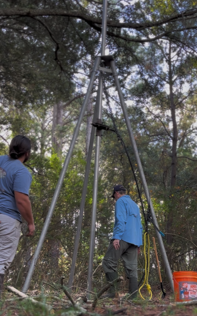
Once the core barrel has reached its final depth, the vibrating head is removed and excess core barrel is cut off prior to retrieving the core. Water is added to the top of the core until it reaches the top of the barrel. A screw lock pressure cap is applied to the core barrel to pull a vacuum on the core’s contents. Now the core is able to be retrieved by pulling it out of the earth vertically using a come-along winch centered above the barrel with a tripod.
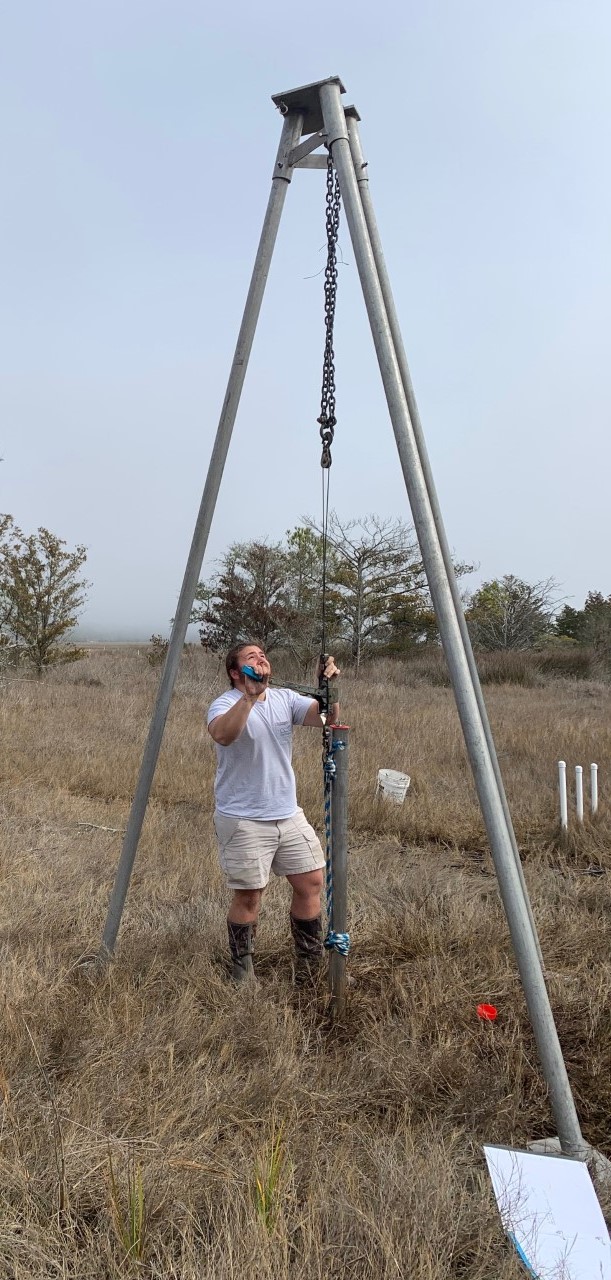
Once the core has been removed from the ground, fast action is necessary to cap the opposite end of the core barrel to ensure contents remain in place. Finally, the core barrel is hauled away to be further processed at the lab.
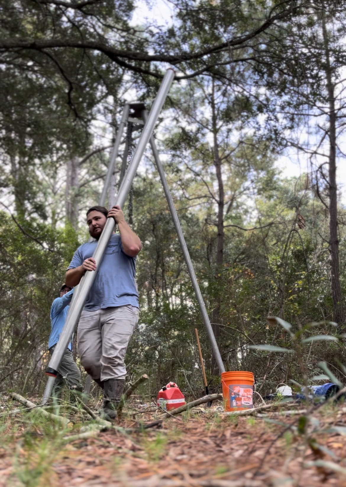
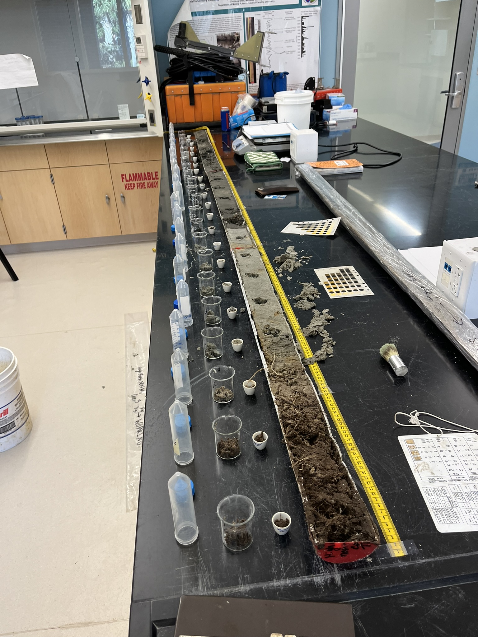
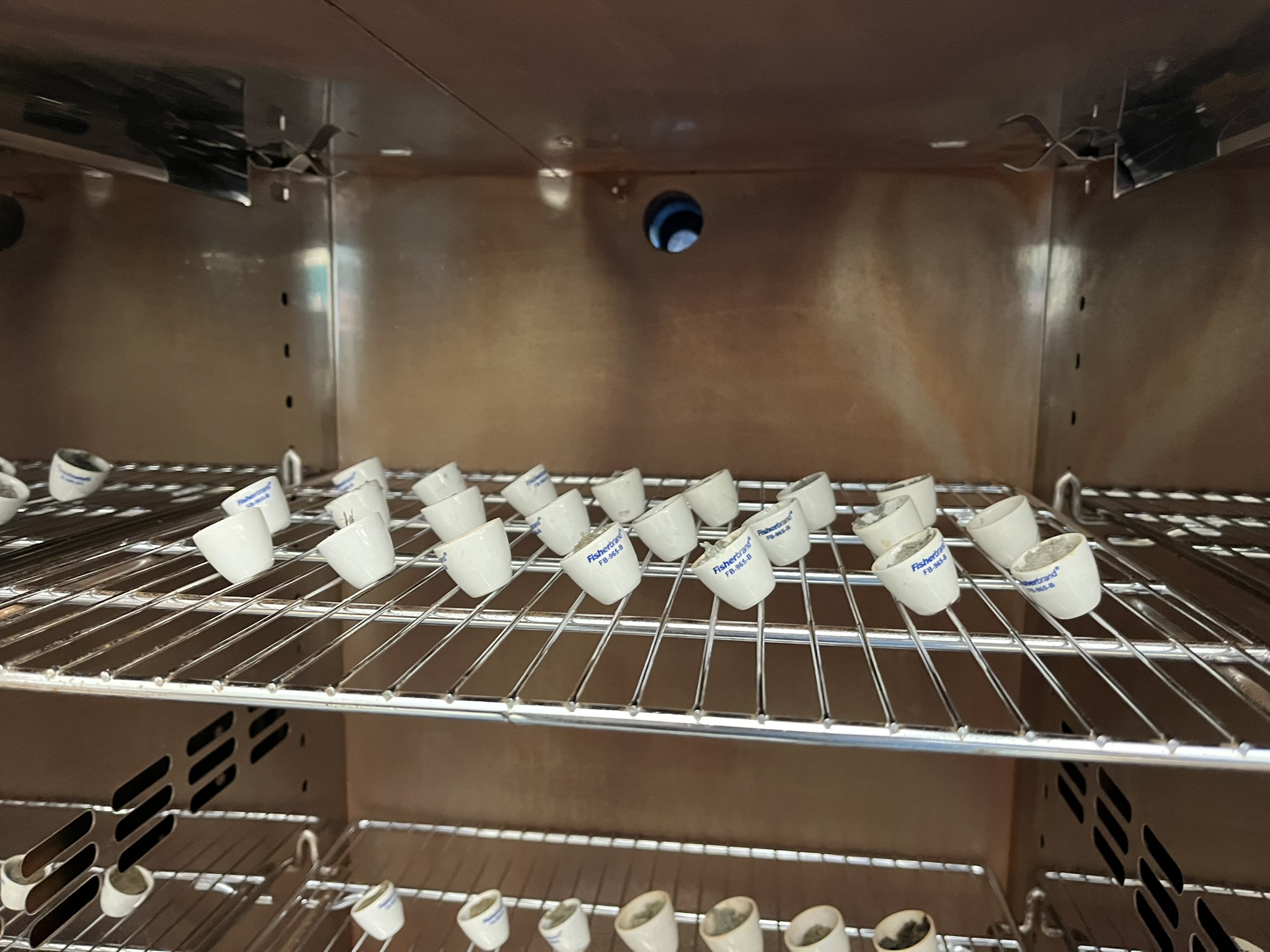
In total, five cores were taken from the study site, four along transect Z, and one in the middle of transect Y. A core was retrieved from each ecological zone; low marsh, high marsh, and maritime forest. Due to the high marsh representing the greatest mixing zone between salty and fresh groundwaters, three cores were taken at various locations to ensure adequate geologic description. Basic descriptions of each core included describing soil color and texture at each layer and noting the presence of fossils or other anomalies. Further analysis included subsampling the core at 15-centimeter intervals to analyze the percent water content, percent organic matter, and grain size of the material. To ascertain values of percent water content and organics, sediment was first loaded into small crucibles weighed, and dried for 24 hours at 221 degrees Fahrenheit. Samples were reweighed and the percent difference was attributed to lost water content. Next, the samples were placed in a muffle furnace and fired at 1,022 degrees Fahrenheit for 4 hours to render any organic material to ash. Again, the samples were reweighed and the percent difference in weight was attributed to the loss of organic material.
To prepare samples for grain size analysis, organic matter must be removed. Hydrogen peroxide was added to the sediment in a beaker and agitated. This reaction was allowed to continue overnight before excess hydrogen peroxide was removed by boiling the sample on a hotplate. Next, shell material needed to be stripped from the sample. Since shells contain mostly carbonate structures an acid wash of 10% sulfuric acid removed this material from the sediment. After continuing overnight, the acid was diluted with deionized water and washed out of the sample by a process of centrifuging and further diluting the sample. Finally, samples were ready to be analyzed by a laser particle size analyzer. This method uses an optical laser to detect obscuration values (how much the laser’s light is obscured i.e. bigger grains, bigger obscuration) which is more accurate than traditional methods of passing the sediment through a series of fine sieves to obtain percent grain sizes. Grain size analysis is essential for geologic description as it is the gold standard for objective characterization of geologic components.
Piggybacking off the prior analyses, falling head permeameter tests are used as a laboratory method of characterizing how groundwater flows through specific types of sediment. Major soil classifications identified by the grain size analysis were subjected to a permeameter test. A falling head permeameter is a benchtop device that has a tall, graduated chamber connected to another chamber at a higher elevation by a hose. The sediment sample is loaded into the graduated chamber and tamped down to closely resemble the in-situ geology of the site. A volume of water is added to the higher chamber which creates the “head”. The tube between the two chambers is opened and the head begins to “fall” through the sample. This operation is timed and continues until the head has been recovered after passing through the sediment sample. This yields a value with units of volume over time. Once the volume of water and volume of sediment is reconciled the final measurement contains units of distance over time, essentially speed. This speed value is known as hydraulic conductivity and is critical for the next analysis, calculations of Darcy’s Law.
Henry Darcy was a hydraulic engineer who existed during the 19th century. He hailed from Dijon, France, the birthplace of Dijon mustard, and is notably remembered for his law that describes the relationship between a fluid and its movement through a porous medium.
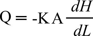
For this application, Q will represent the rate estimation of groundwater movement between wells along transect Z. Term A will be the two-dimensional area of the well screen underground, dH is the recorded height of the water table within the well, while dL is the horizontal distance between the wells. This calculation will provide some rough estimates of Darcy flow at specific points in time, we can then track how major hydrogeologic forces like storms and larger tides may accelerate or diminish groundwater movement.
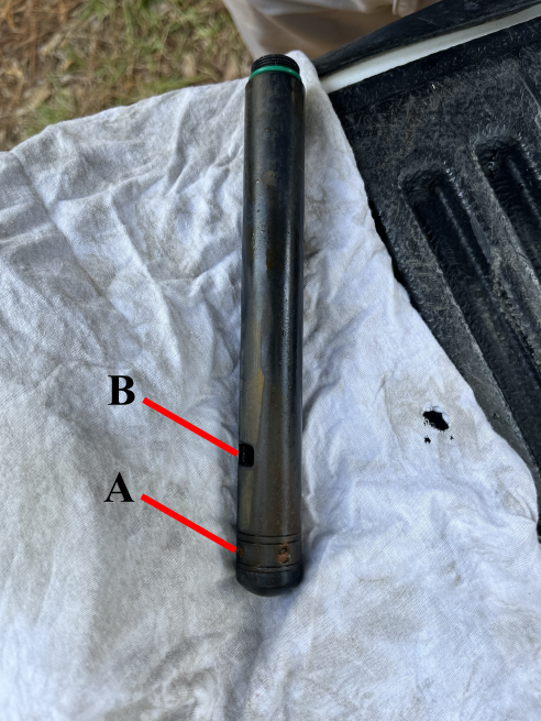
We’ve mentioned water table elevation several times now without addressing how it will be measured. While measuring to the water table in the well could be accomplished with a simple tape measure, this does not provide high enough resolution data that would be worth anyone’s time analyzing. Our 21st-century approach is to deploy sensors underwater in the well that measure the pressure of the water above the sensor. With some quick math to calculate the pressure of water and compensation to include the pressure of air, an accurate elevation measurement of the water table can be achieved. For this study, we deployed three Solinst LTC5 leveloggers, and set them to take a record every twenty minutes. In addition to water level, these sensors record water temperature and salinity. These measurements are not only valuable for Darcy’s Law calculations but will also contain the fingerprints of hydrogeologic forces such as rain and storm surges from major storm events and the effect of tides pushing the water within the marsh soils. In order to untangle these hydrogeologic forces a statistical method known as ensemble empirical mode decomposition can be used. This method uses a moving average to deconstruct the underlying signals comprised in the mother (original) signal. We can then parse through the output, known as residuals, to find sub-signals that align with tidal and precipitation records.
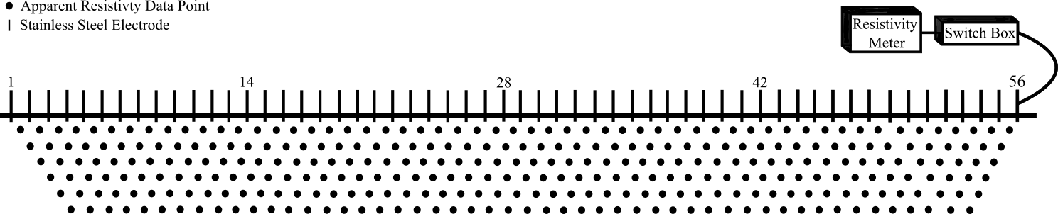
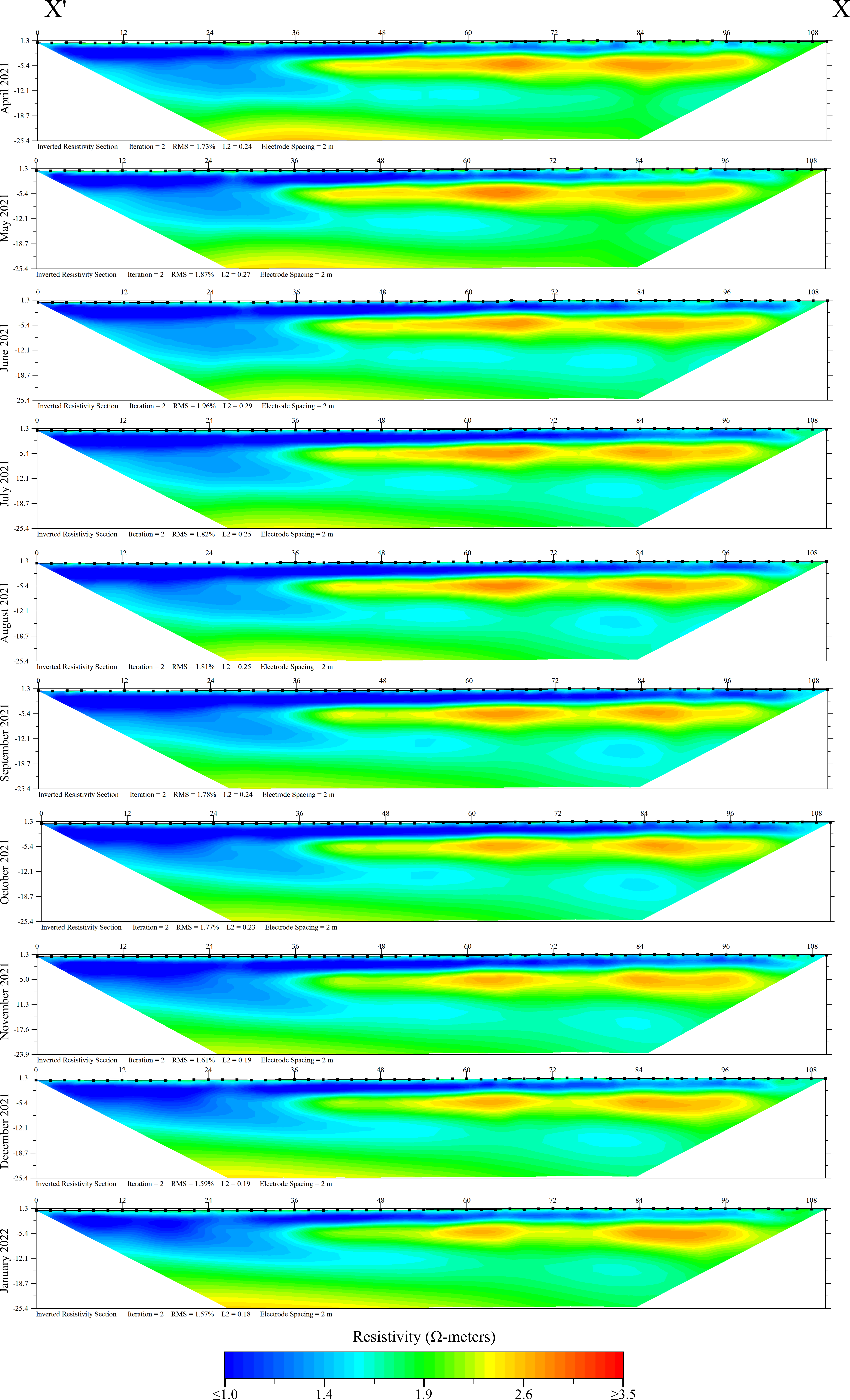
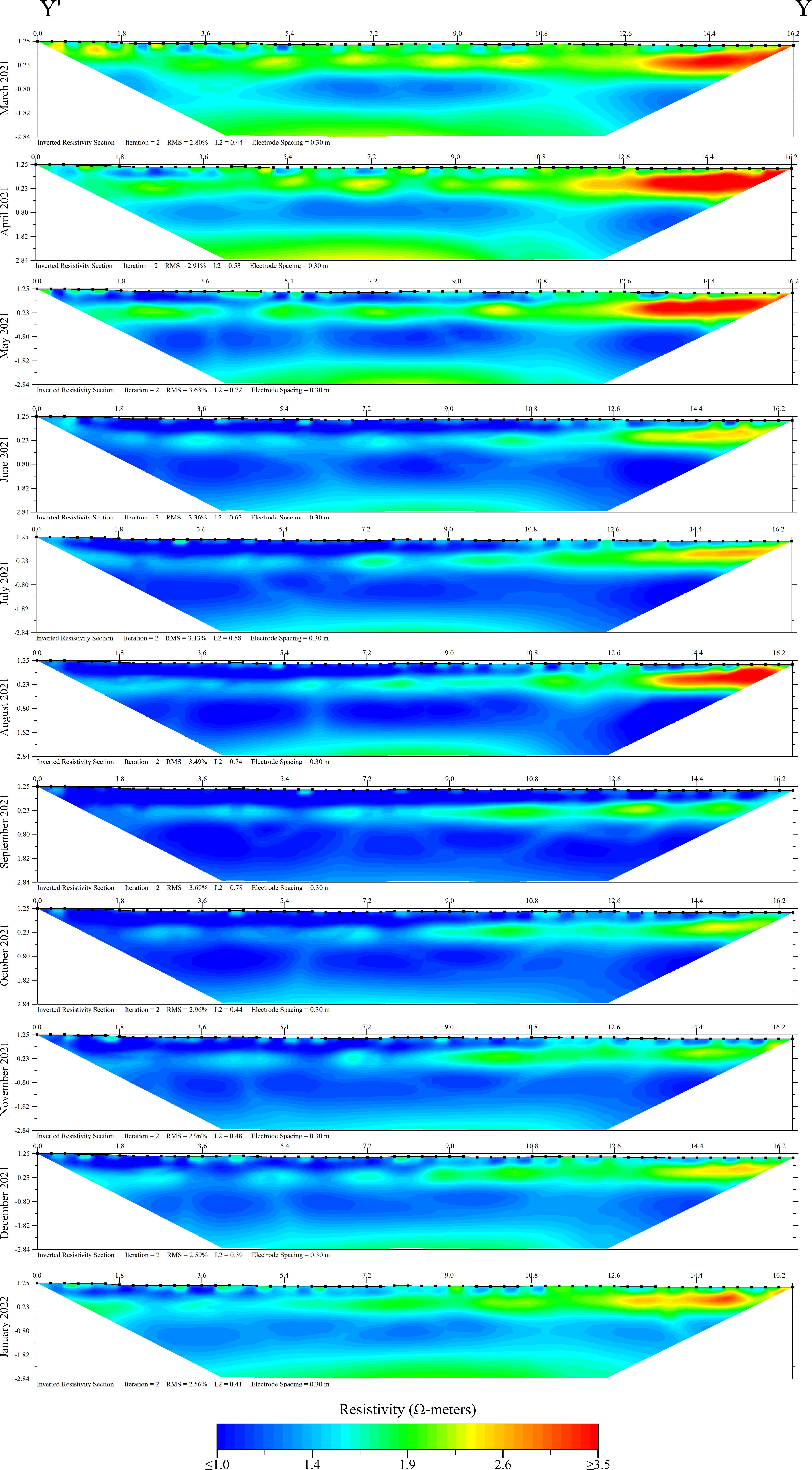
Electrical resistivity surveys were used as a geophysical tool to assist in imaging groundwater and identifying potential mixing zones across the study site transects. Electrical resistivity (ER) is a method that uses a series of electrodes and applied electric currents to measure the resistive properties of the earth. The electrodes are 56 stainless steel spikes inserted into the ground, and electricity is applied by a long cable with 56 graphite terminals spaced throughout. This apparatus is connected to a switchbox and main head unit which systematically selects a pair of electrodes in the array to make a measurement. Once selected, the first electrode receives electricity at a known voltage, and the second electrode in the pair waits to receive the remaining voltage as it passes through the ground. This setup essentially creates a basic circuit that uses the earth material underneath the survey as a resistor. The resulting data point is an “apparent resistive” value located along the arc the electrical current travels on between the two points. The head unit and switch box cycle through the entire 56-electrode array to create a matrix of apparent resistivities.
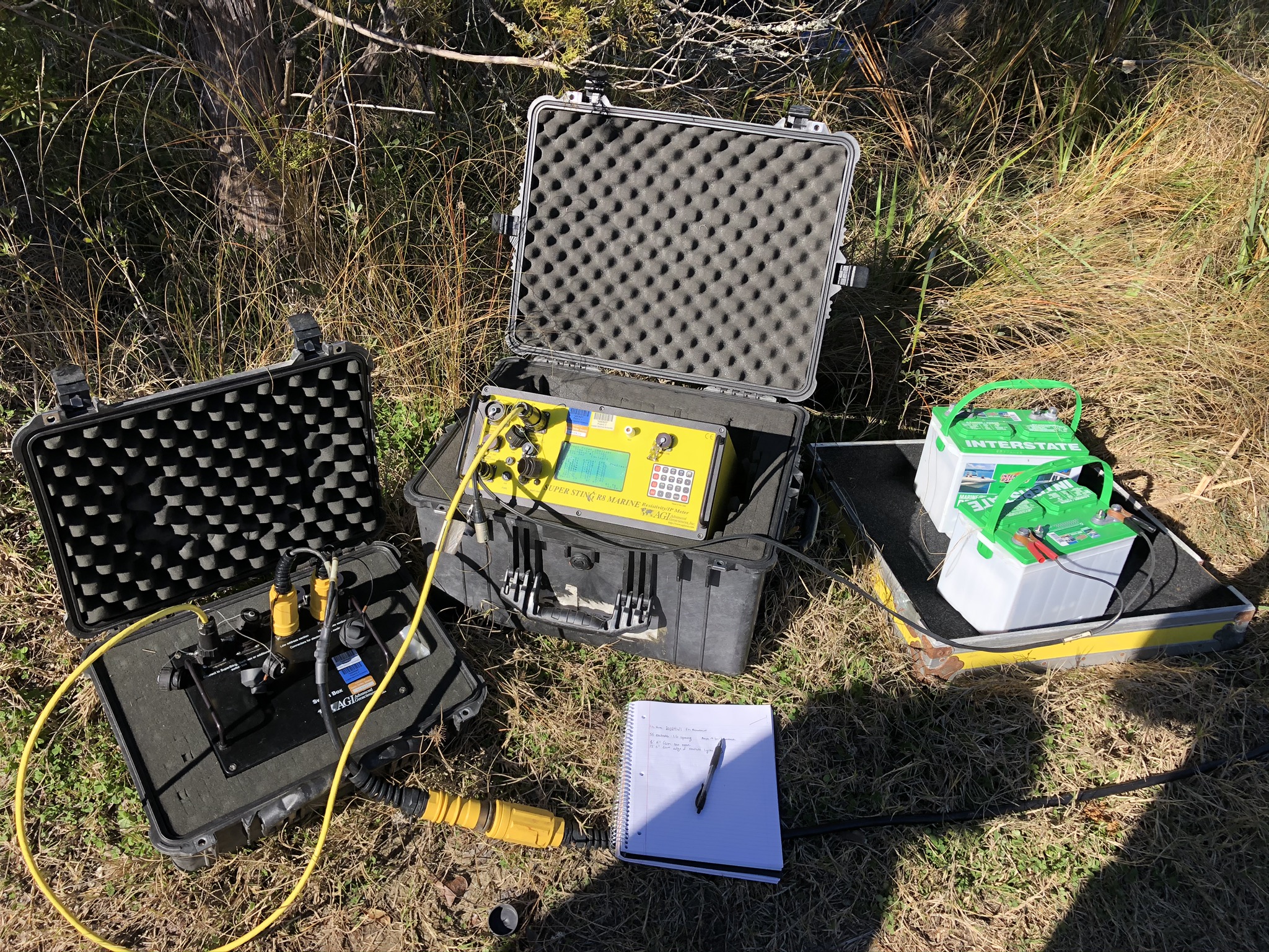
In traditional approaches, this method can be used to identify large buried objects, gaps or caves underground, large regions of conductive ore, or for groundwater exploration. When this technique is used in a salt marsh environment, there are a few assumptions that must be made due to the conductive nature of saltwater and the overall saturation of the sediment. Here it’s believed that the resulting ER signal is sensitive to changes in geology, porosity, sediment texture, and salinity of waters within the sediment. We use this technique in a time series format, completing a survey monthly at the exact same point to identify any seasonal or event-driven changes in the resistivity signal. Since the surveys are stationary through time, we control for any changes in geology, meaning any changes in resistivity signal must be due to the amount of groundwater in the subsurface or the salinity of that groundwater.
Content beyond this point is preliminary, final Results and Discussion will arrive late April 2024
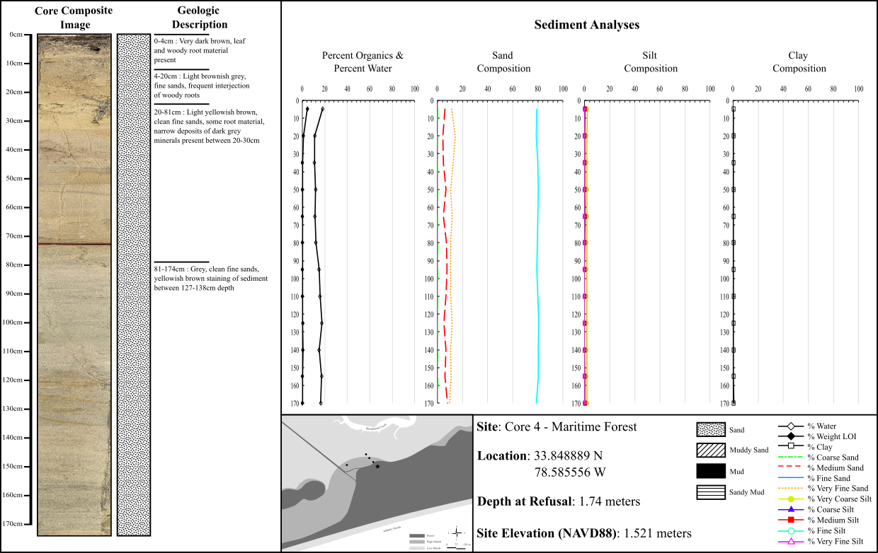
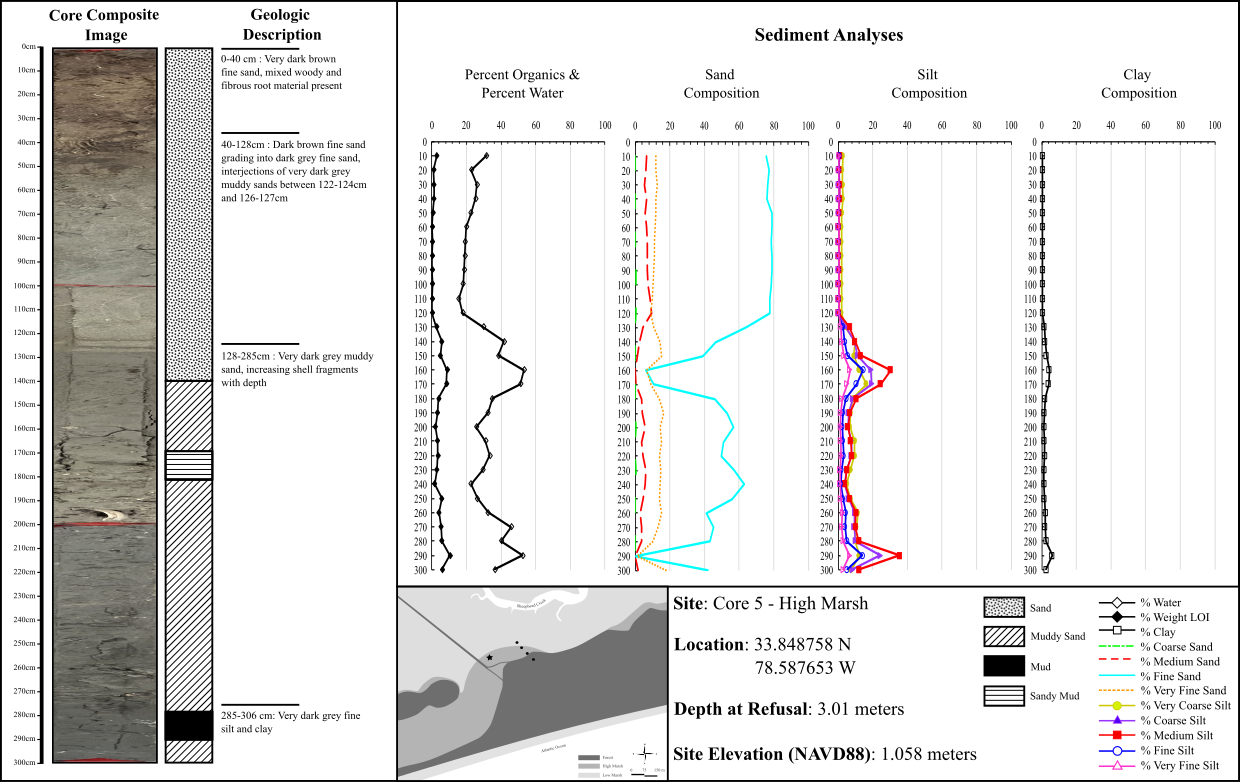
Four major sediment types were identified through grain size analysis; sand, muddy sand, mud and sandy mud. Sediment types such as sandy mud can be thought of as a muddy sediment that contains a notable fraction of sandy sediments. Ultimately these sediment types describe the overall distribution of grain size within a specific section of the core. Listing these sediment facies from high to low permeability, sand would be first, followed by muddy sand and sandy mud, with mud being the least permeable sediment type due to the tightly packed fine-grained nature of the sediment.
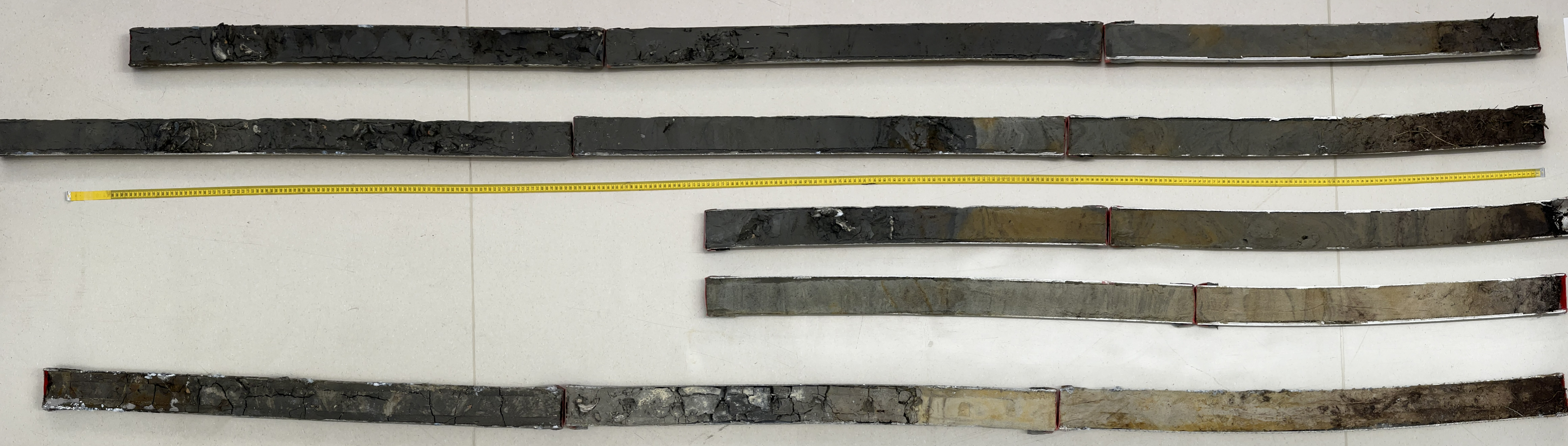
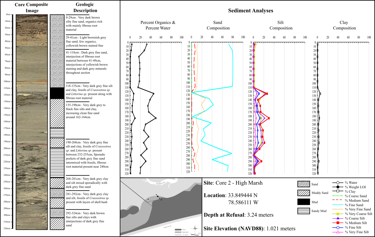
Core 1, from the low elevation saltmarsh, reached the second greatest depth out of all the cores taken, with bottom sediments laying approximately 9.7 feet below the marsh surface. Upper sandy sediments gave way to more muddy soils with depth, which also contained several estuarine fossils such as periwinkle snails and oyster shells. Sandy layers retained much less water and organic material than their muddy counterparts.
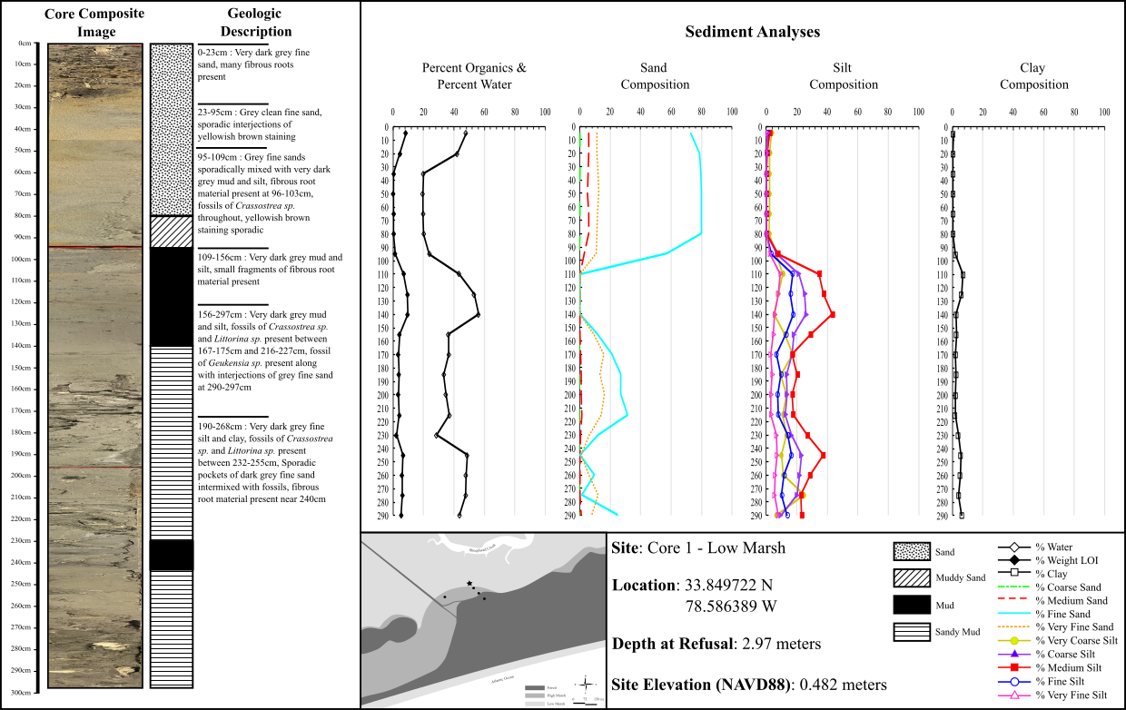
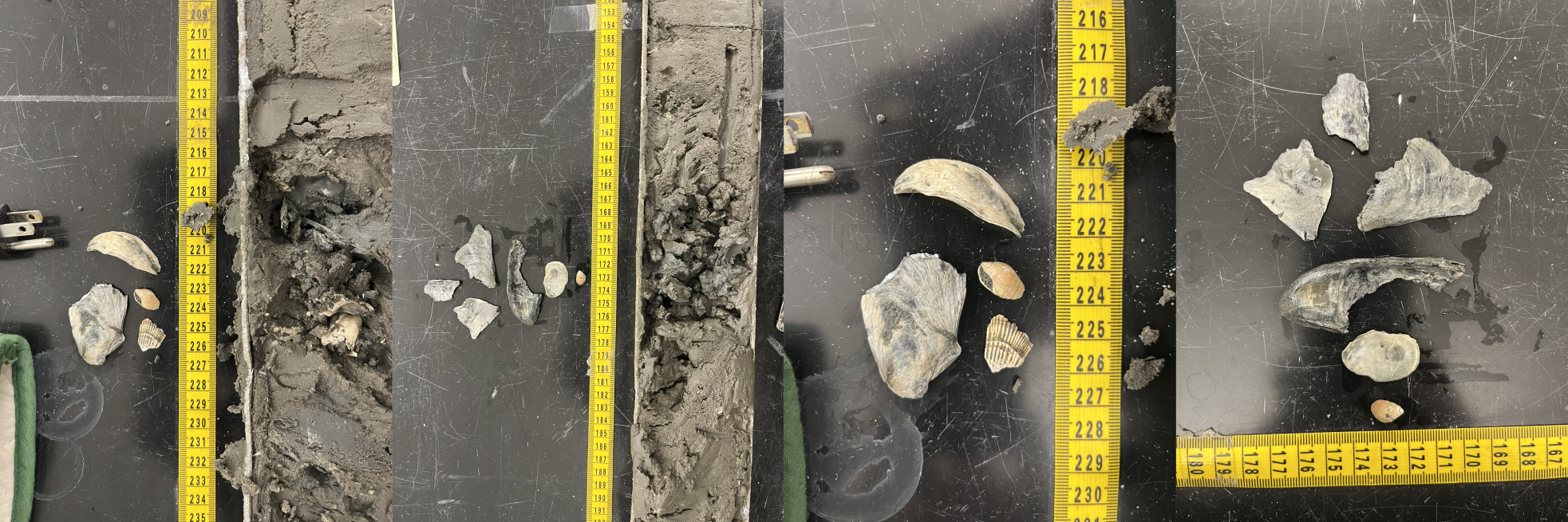
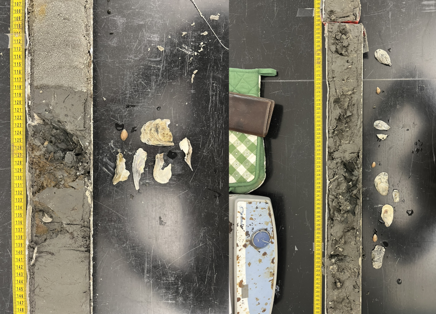
Core 2 retrieved sediments from the greatest depth, 10.6 feet below the marsh surface. Upper sediments maintained the same pattern as Core 1 with sandy sediments atop muddy sediments, however frequent flips between sandy and muddy type sediment was common with depth. More oyster and snail fossils were found in muddy estuarine-type sediments within the core.
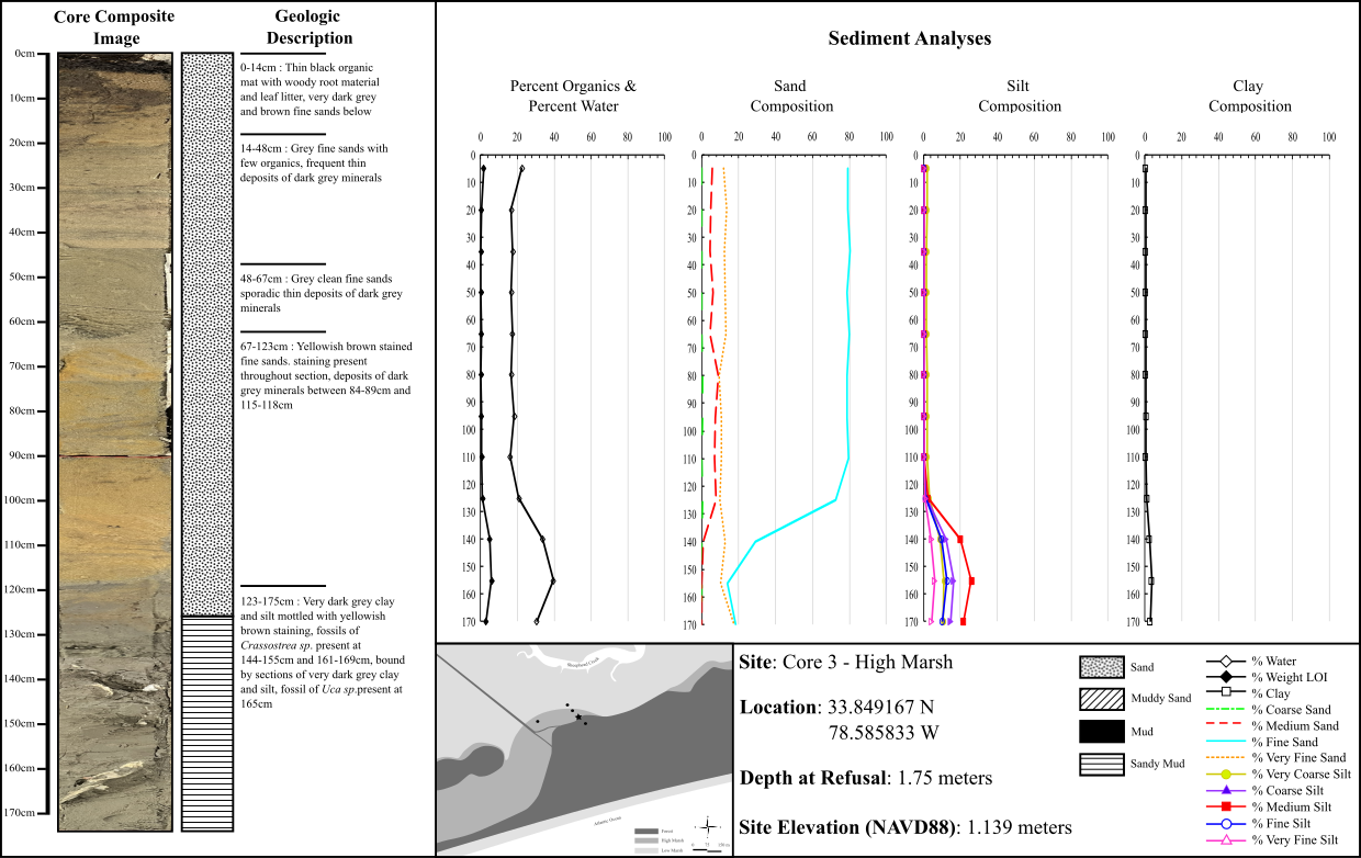
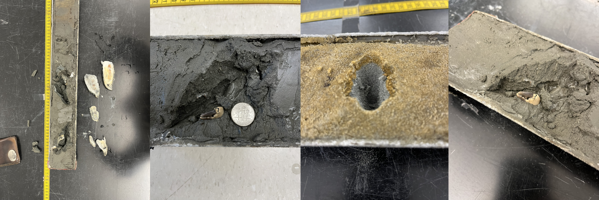
Core 3 was located directly adjacent to the high marsh well and recovered 5.7 feet of material. With shallower penetration and increased elevation as the core transect enters the island, a simpler geology emerged. The upper ¾ of the core contained sandy sediments with the last quarter revealing a sandy mud. Fossils of oysters were found at the lowest reaches of the core and an intact claw from a fiddler crab-like species.
Core 4 reached approximately the same depth as Core 3 and recovered 5.7 feet of maritime forest material where sand was the predominant soil type. A narrow mat of leaf litter and root material was present at the top of the core but did not proliferate much deeper than 1 foot in depth.
Core 5, located in the middle of Transect Y rather than along Transect Z, gathered material from 9.9 feet below the transect which was similar in composition to Core 2. Upper sandy sediments became increasingly muddy with depth, and broken fragments of oyster fossils were found within muddy estuarine sediments.
Over the course of three years and three transects, 29 electrical resistivity surveys were collected. Surveys along transects X and Y were co-located and collected concurrently between 2021-2022, while transect Z’s data was gathered during the 2023 field season. Overall, soil resistivity was greatest towards the island and diminished with increased distance into the saltmarsh. These higher regions of resistivity were confined between 1.5 and 9 feet below the marsh surface at their widest and began to pinch out into the marsh.
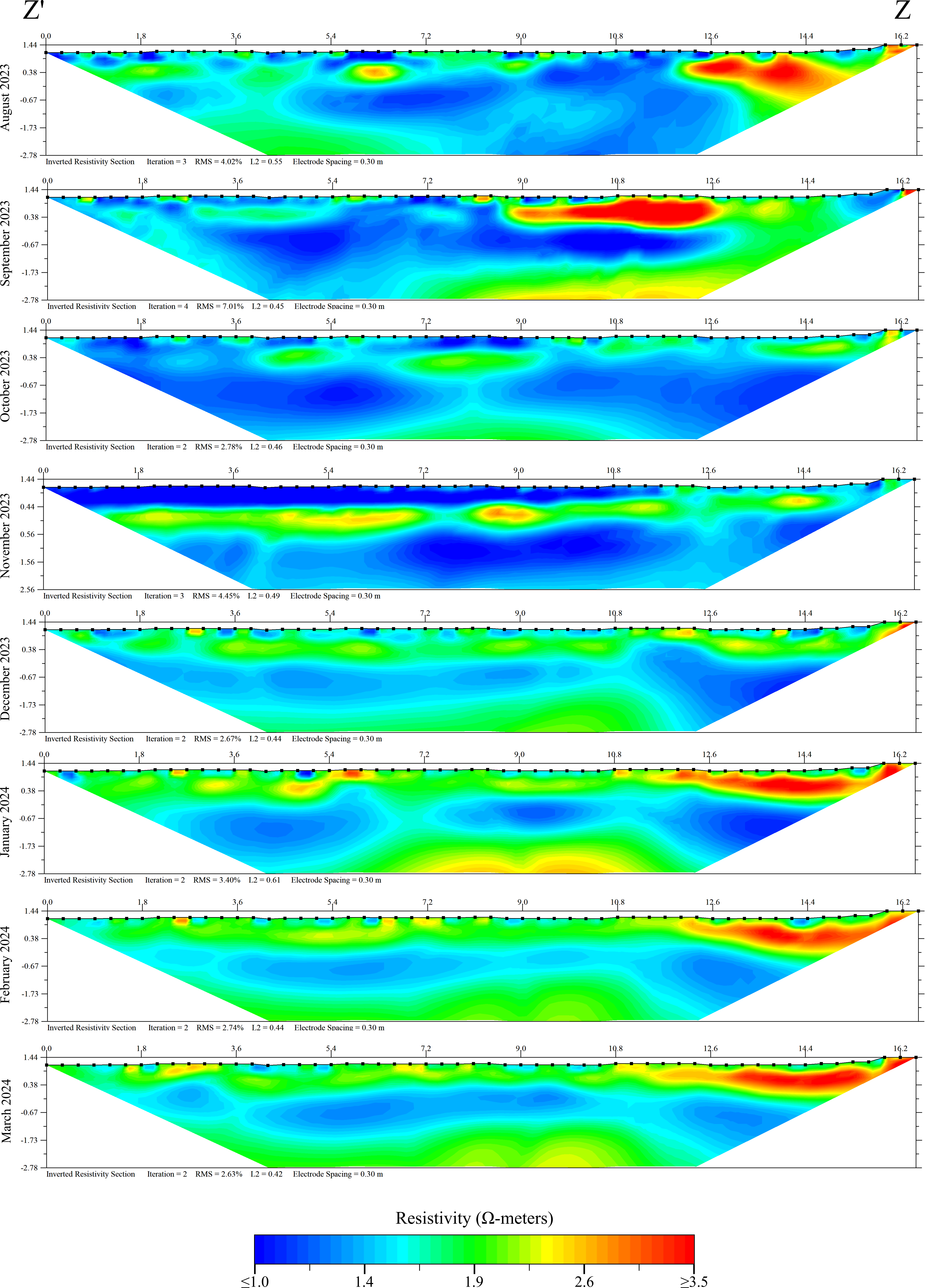
Results coming soon!
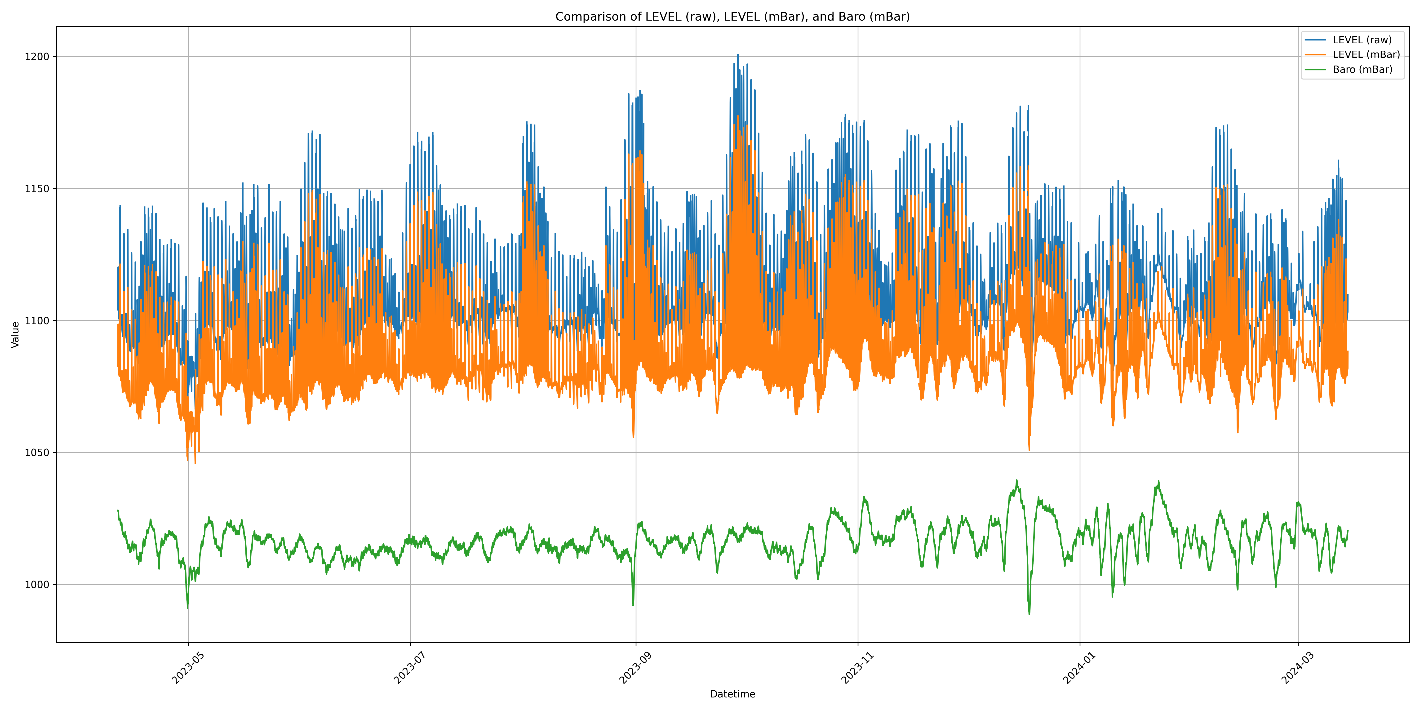
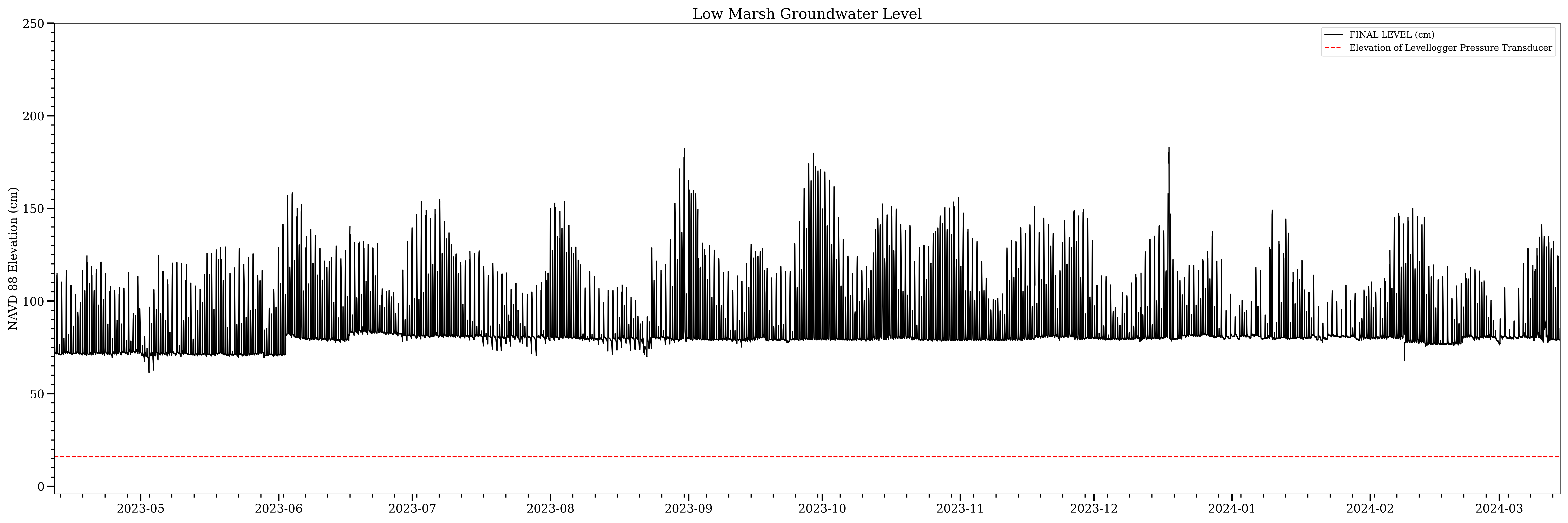
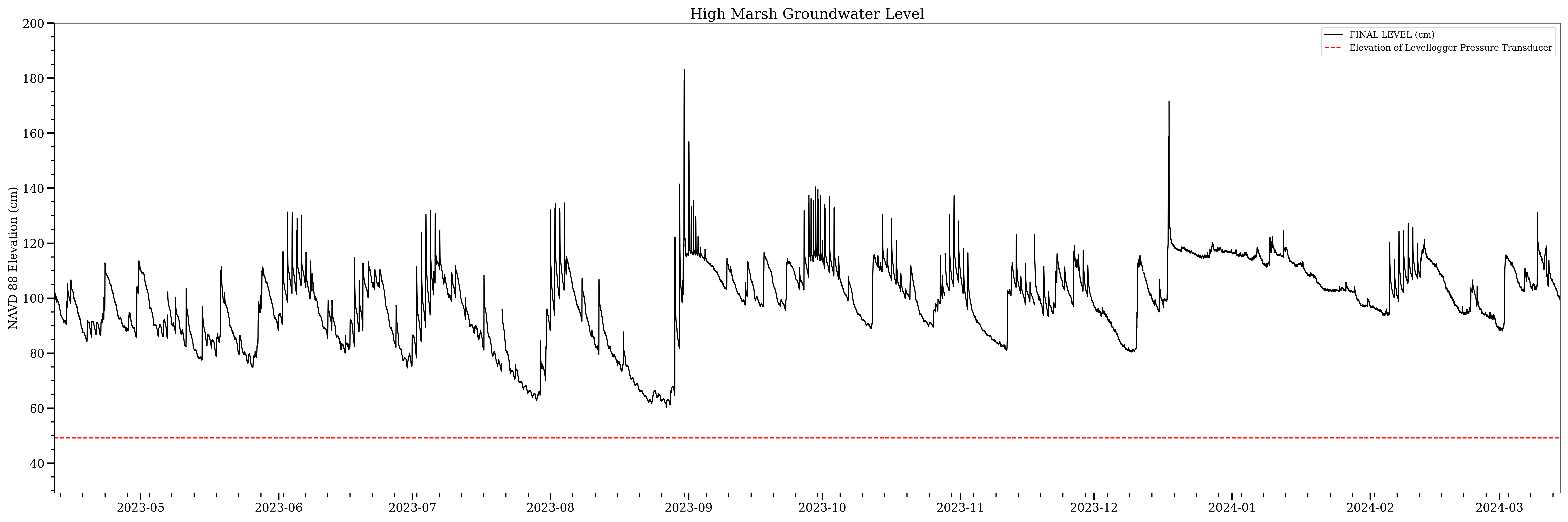
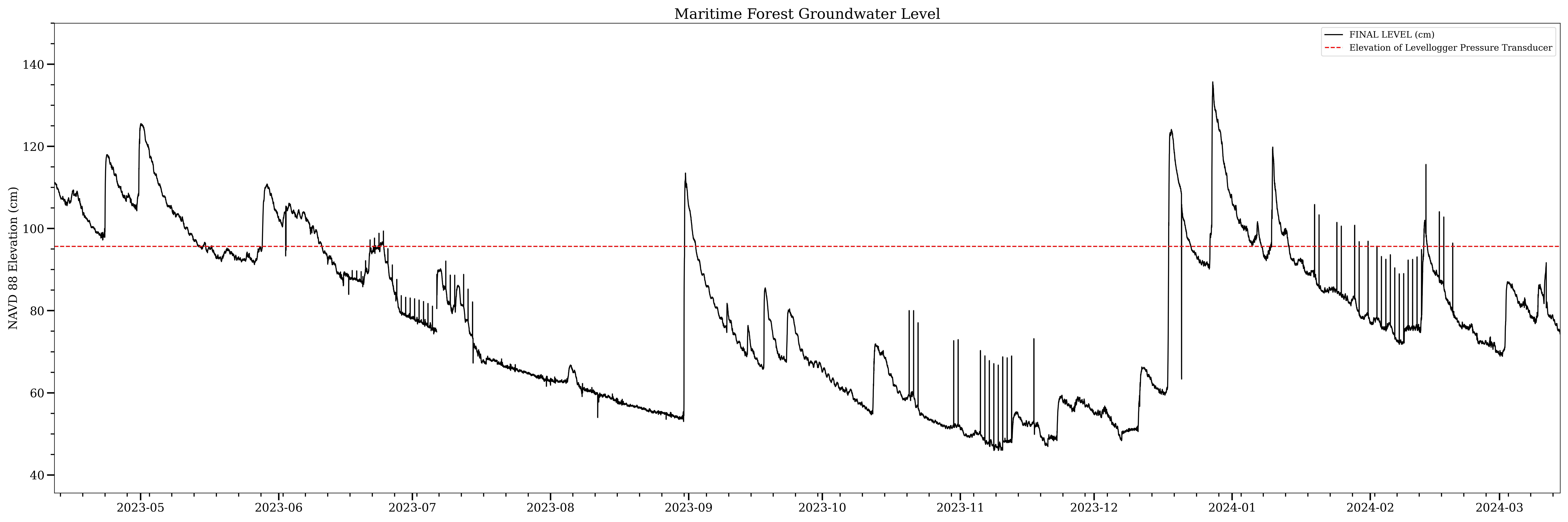
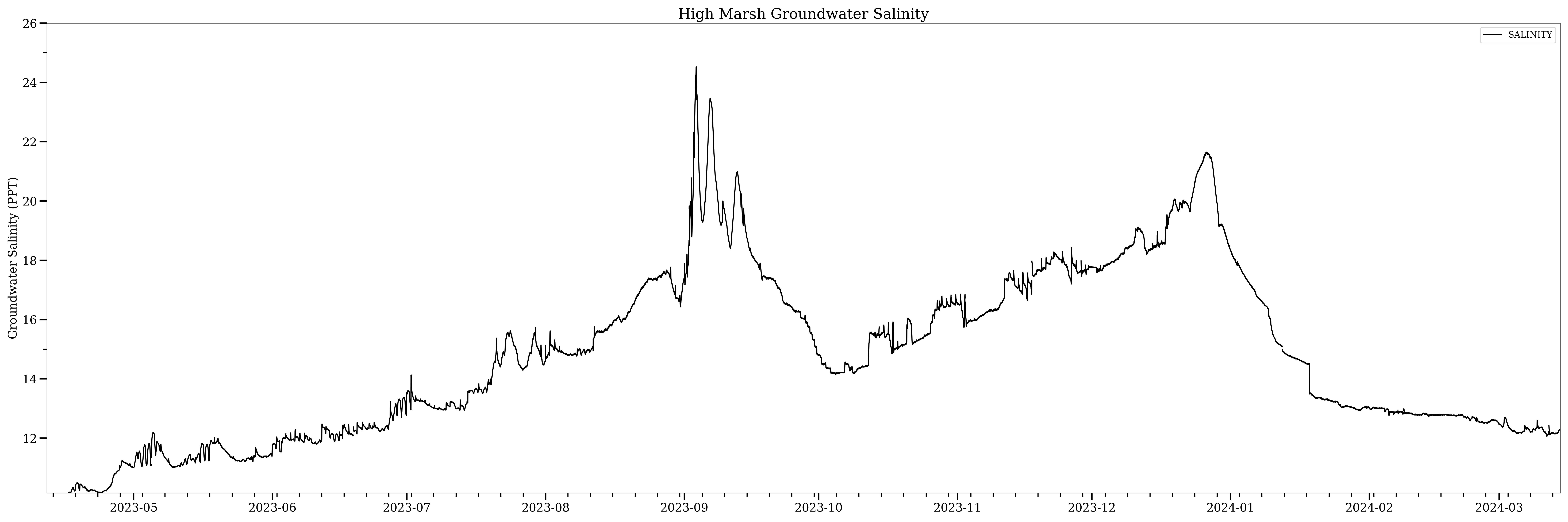
24,331 measurements of the groundwater were taken over the period from April 11, 2023 to March 14, 2024. Of the three wells, the low marsh well exhibited the greatest amount of variability. A strong tidal component can be observed throughout the data, this tidal signal is less pronounced moving into the high marsh well and is only present for brief periods in the maritime forest well. Major precipitation events following Hurricane Idalia (Aug. 30 - Sept. 1) and a significant nor'easter storm (Dec. 17) can be observed in all datasets.
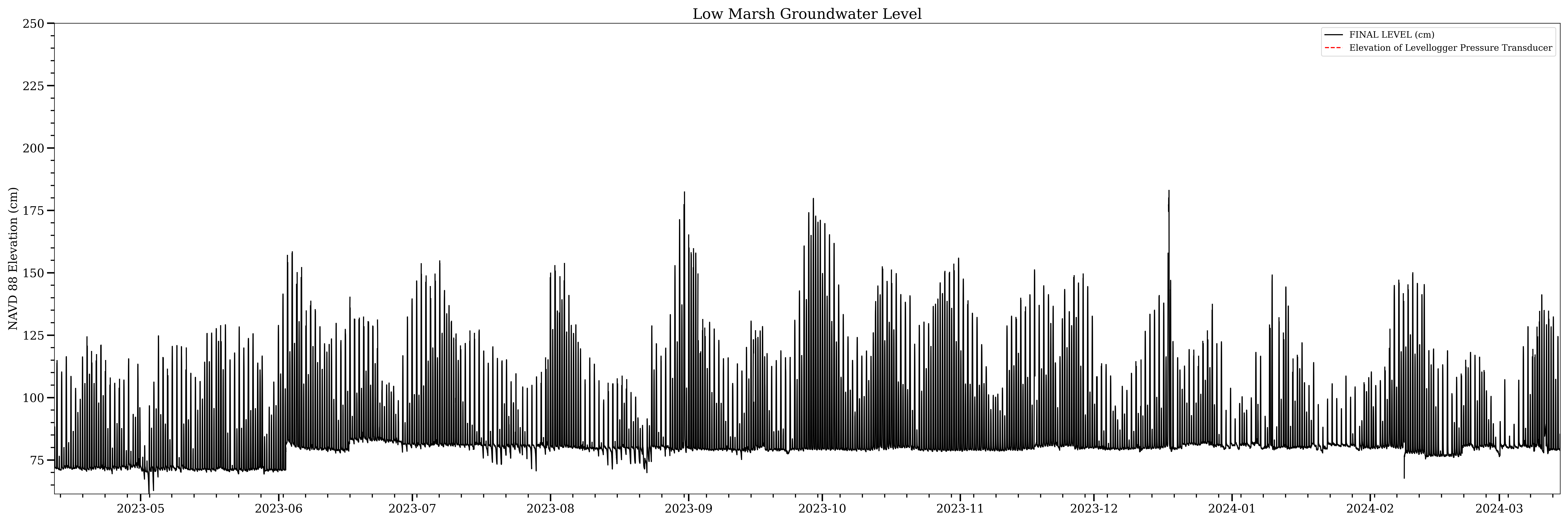
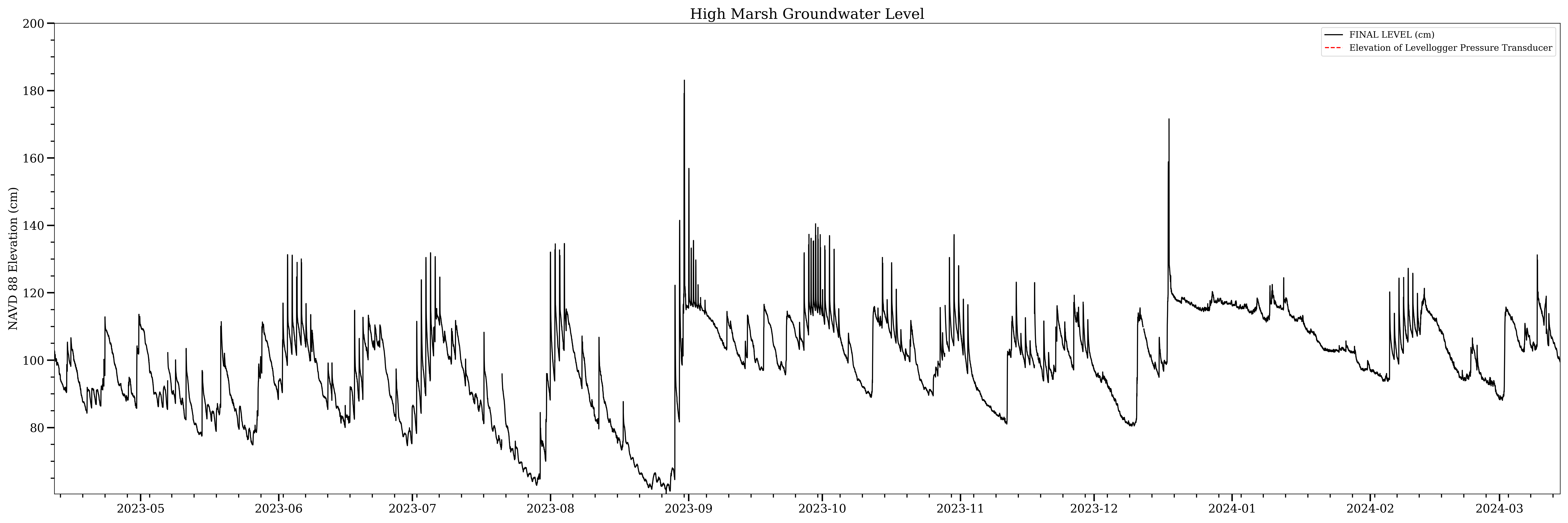
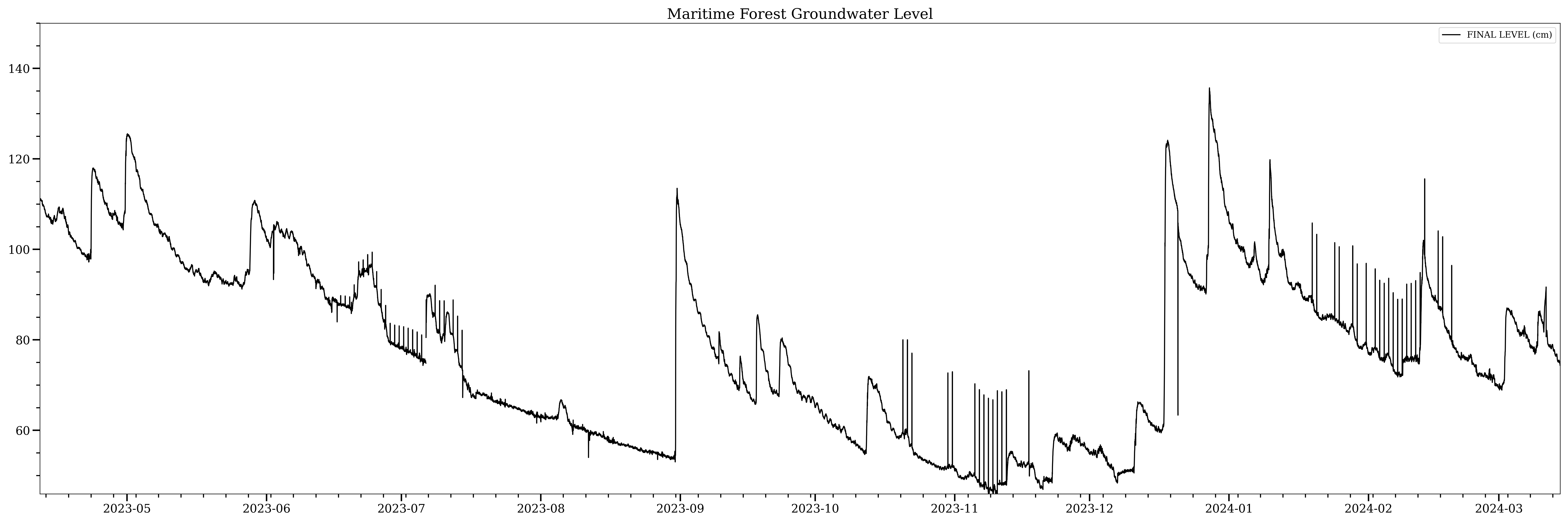
As previously described, the water level is measured by a pressure transducer onboard the levelogger suspended within the well. The red dashed line in the following graphs marks where the levelogger is hanging relative to the water level. The low marsh well maintained the greatest average amount of water above the sensor while the forest well experienced times when there was little to no water above the sensor (although this could be an instrument error, currently being investigated)
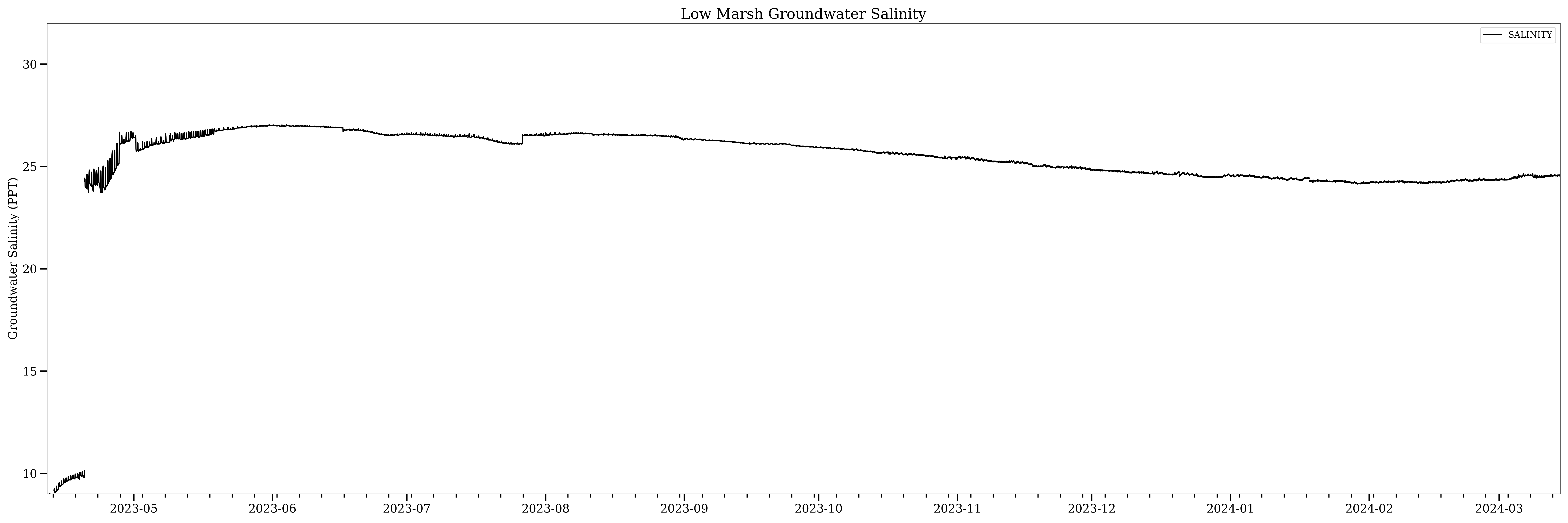
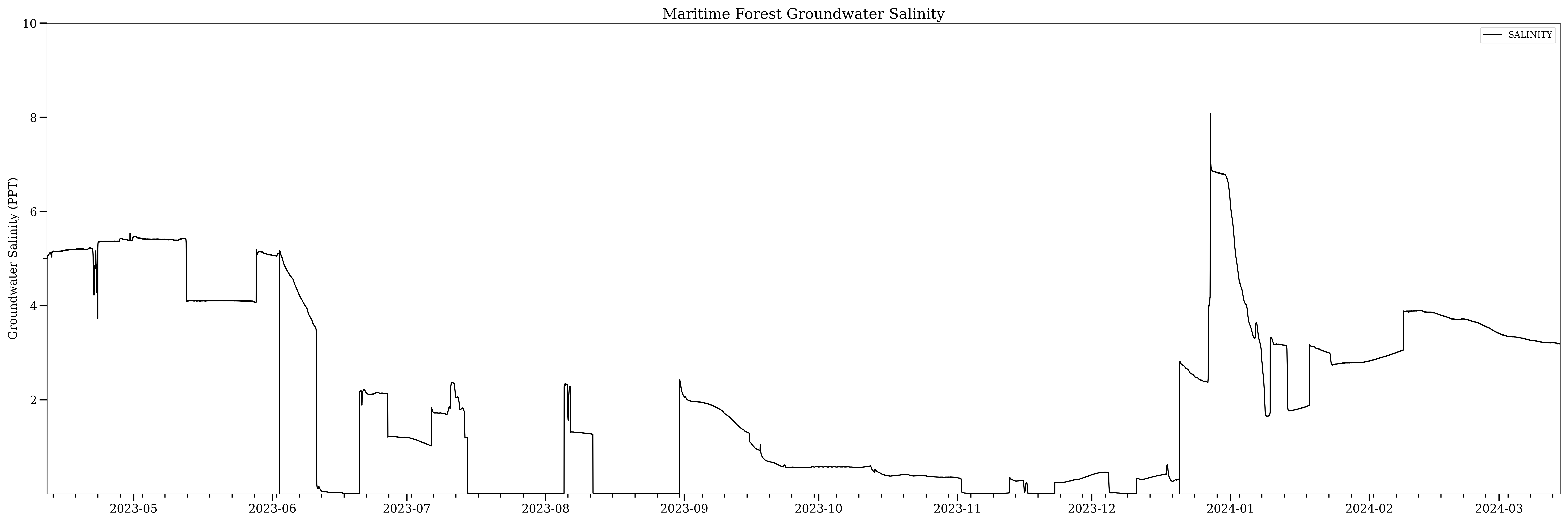
Salinity values were as expected, with the highest values in the low marsh well, mixed values in the high marsh well, and the freshest/lowest values in the forest well. What was not expected was the step-like nature of the maritime forest well and the first data installment of the low marsh well. Current literature suggests that any measurement of groundwater salinity via the groundwater well method may be inaccurate due to the stratification of water within the well volume. This could explain step-like functions as waters of various salinity pass over the stationary levelogger with rising and falling levels.
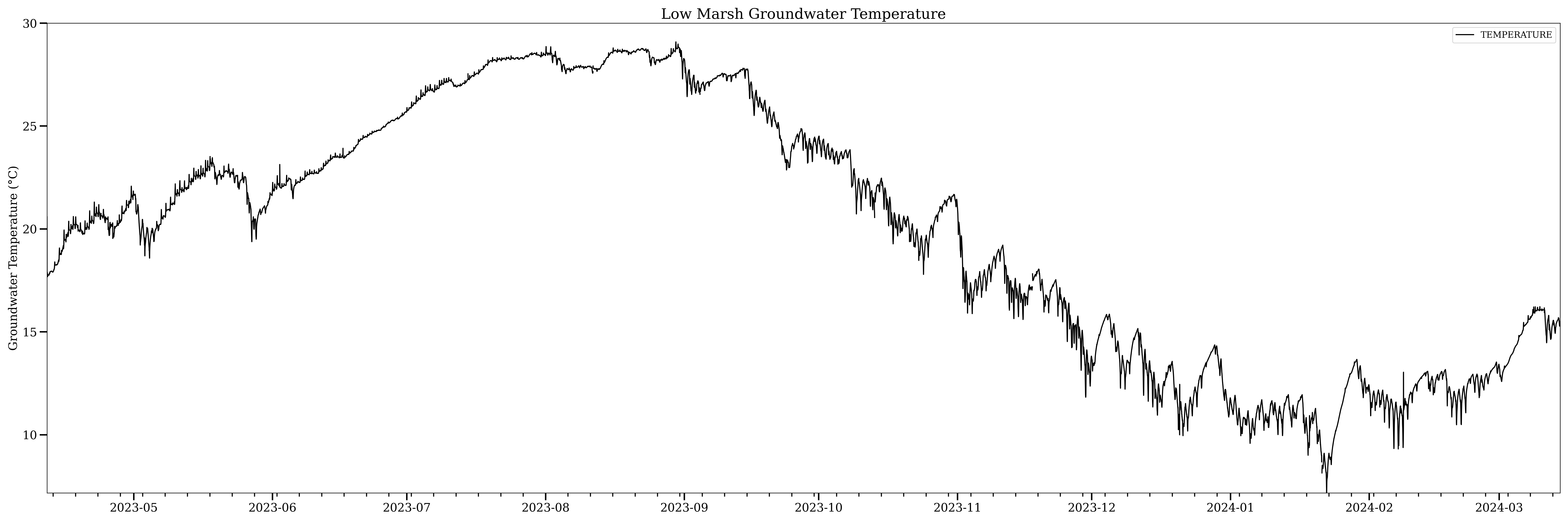
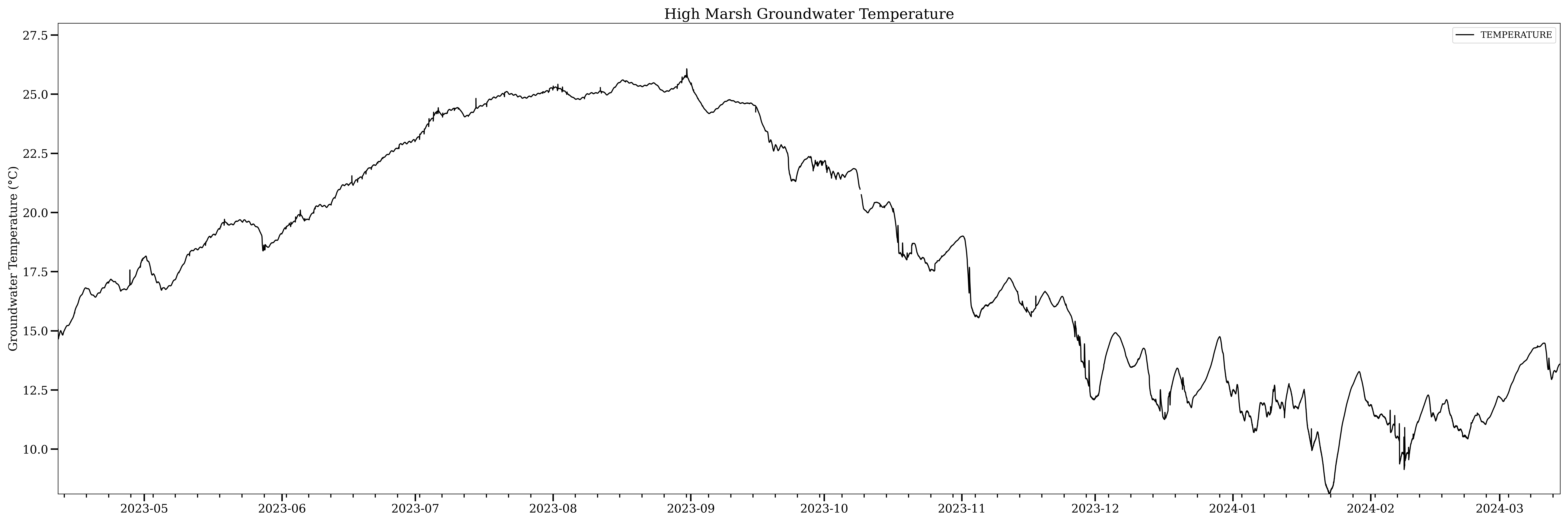
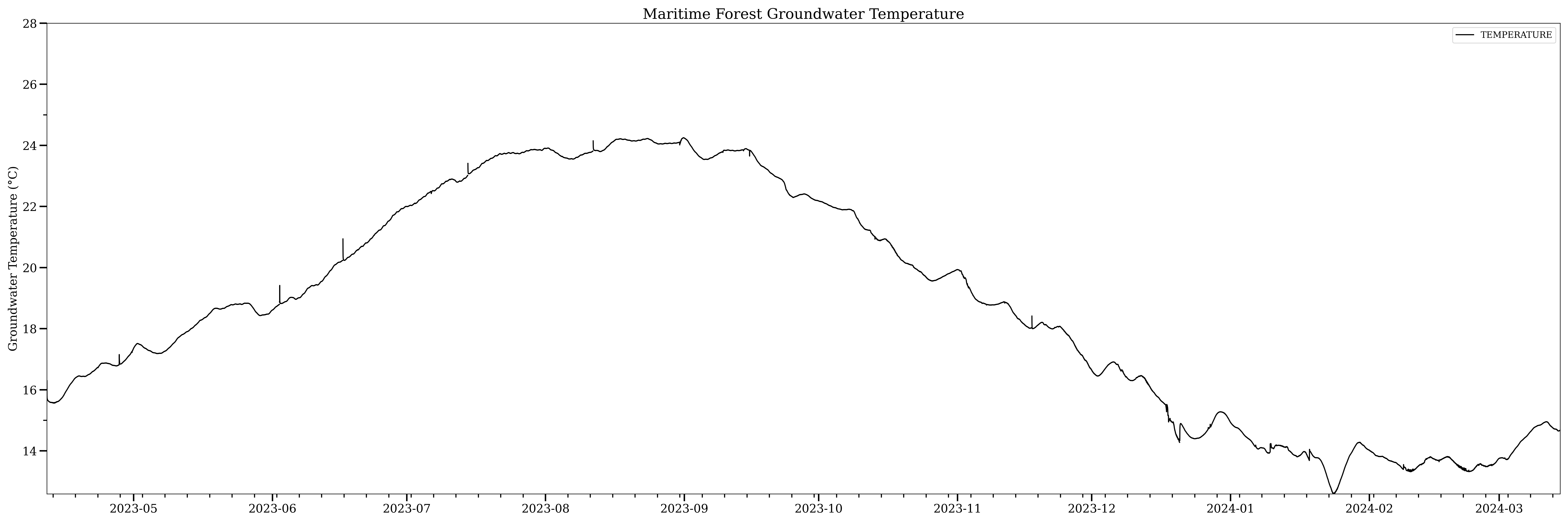
Similar to groundwater salinity, temperature is predisposed to inaccuracy due to the stratification of waters within the well volume. Additionally, the temperature of groundwater within the well is more than likely a reflection of air temperature. This is due to the well volume being exposed to the atmosphere, stripping away the insulating properties of the earth. If you've ever drank from a well on a hot summer day, you can readily tell the difference in groundwater and air temperature. However, these are very shallow wells, and such stratification between air temperature and groundwater temperature can be observed in the low marsh data set, where tidal fluctuation pushes the stratified layers across the sensor constantly, resulting in the jagged or saw-tooth pattern.
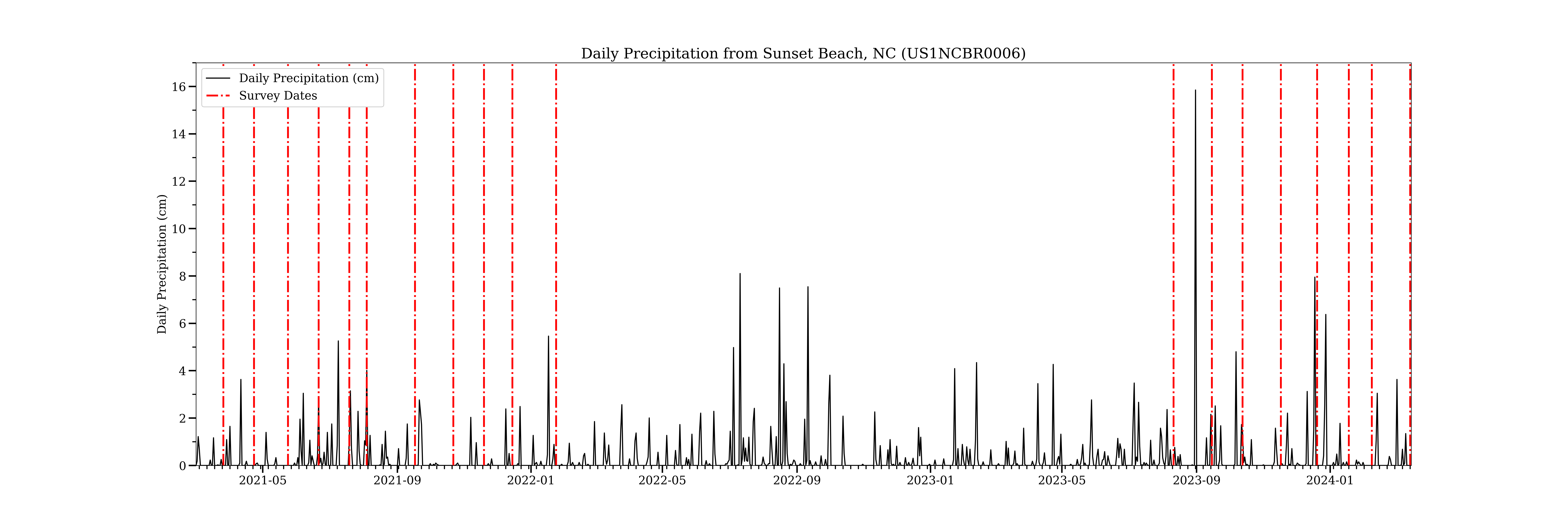
We briefly touched on major storm events impacting the level data in each well. For data analysis, a constant record of precipitation on the site is needed. Ask anyone who has spent a significant amount of time during the summer in the southeast and they will tell you rainfall, especially afternoon rainfall, is hyperlocal. Rain could accumulate 1-2" in one locale and be bone dry >1 mile away. This premise highlights the need to select rainfall data from the nearest rain gauge possible. The common practice when searching for data is to search government repositories and local offices first, however in the case of high-quality meteorological data, the nearest station is located 8 miles away at the North Myrtle Beach Airport. A CoCoRaHS (Community Collaborative Rain, Hail, and Snow) gauge is located only 2.5 miles away in neighboring Sunset Beach, NC. While citizen science is a noble effort and in this case provides tangible utility, it's best to utilize this data with the motto "Trust But Verify" in mind. To do this CoCoRaHS daily rainfall totals were compared to the official rainfall totals from both NOAA's Springmaid Pier station and NWS' North Myrtle Beach station. Small differences (>.1") were seen between datasets and could be attributed to the hyperlocallity discussed above. Furthermore, rainfall events could be verified by observing a corresponding drop in barometric pressure.
Coming Soon!